The Functional Mock-up Interface (FMI) is a free standard that defines a container and an interface to exchange dynamic models using a combination of XML files, binaries and C code, distributed as a ZIP file. It is supported by more than 170 tools and maintained as a Modelica Association Project (MAP FMI). Releases and issues can be found on github.com/modelica/fmi-standard.
Copyright © 2008-2011 MODELISAR Consortium and 2012-2022 The Modelica Association Project FMI.
This document is licensed under the Attribution-ShareAlike 4.0 International license. The code is released under the 2-Clause BSD License. The licenses text can be found in the LICENSE.txt file that accompanies this distribution.
Attention is drawn to the possibility that some of the elements of this document may be the subject of patent rights. Modelica Association shall not be held responsible for identifying such patent rights. All contributors to this specification have signed the Corporate Contributor License Agreement of the FMI Project or the Contributor License Agreement of the Modelica Association.
1. Introduction
1.1. What is new in FMI 3.0
The FMI Design Community has improved the FMI standard to react to new requirements from the system simulation community.
Especially the ability to package control code into FMUs required some workarounds in FMI 2.0. With FMI 3.0, virtual electronic control units (vECUs) can be exported as FMUs in a more natural way. Concrete features to support vECU export are:
-
introduction of terminals to group variables semantically to ease connecting compatible signals,
-
introduction of icons to define a graphical representation of the FMU and its terminals,
-
introduction of Clocks to more exactly control timing of events and evaluation of model partitions across FMUs,
-
introduction of more integer types and a 32-bit float type (see
modelDescription.xml) to communicate native controller types to the outside, -
introduction of a binary type to support non-numeric data handling, such as complex sensor data interfaces,
-
extension of variables to arrays for more efficient and natural handling of non-scalar variables,
-
introduction of structural parameters that allow description and changing of array sizes, even during runtime to support advanced online calibration of control code, and
-
addition of the new interface type "Scheduled Execution" (see Section 5) that allows activation of individual model partitions by an external scheduler, e.g. on real-time platforms.
To allow implementation of more robust and efficient co-simulation algorithms, the following features were added to FMI for Co-Simulation:
-
Early return from a
fmi3DoStepcall, -
the Intermediate Update Mode, and
Besides directional derivatives, now adjoined derivatives of variables can be obtained.
The newly introduced <BuildConfiguration> simplifies the integration of source-code FMUs.
The following features have been removed:
-
The asynchronous mode for FMUs known from FMI 2.0 CS: this mode was not supported by tools and it can be suitably replaced by Co-Simulation implementations that control the asynchronous computation of FMUs via separate processes/threads created for each FMU.
-
The FMI
fmi2SetRealInputDerivativesfunction: replaced by enabling the setting of inputs in Intermediate Update Mode.
Parallel to the new standard features, the FMI Design Community has improved the standard quality by:
-
modernizing the development methodology (e.g. moving to github and following the github process) and a text-based source format,
-
publishing the FMI Standard now primarily as html to support easier navigation within the document and viewing on a wider range of devices,
-
supplying a large set of continuously validated Reference FMUs, and
-
integrating within the FMI Standard only validated C-code, XML and XSD snippets to reduce redundancy and ensure correctness.
1.2. Overview
The Functional Mock-up Interface (FMI) defines a ZIP archive and an application programming interface (API) to exchange dynamic models using a combination of XML files, binaries and C code: the Functional Mock-up Unit (FMU). The API is used by a simulation environment, the importer, to create one or more instances of an FMU and to simulate them, typically together with other models. The FMI defines three interface types:
-
Co-Simulation (CS) where the FMU typically contains its own solver or scheduler,
-
Model Exchange (ME) that requires the importer to perform numerical integration, and
-
Scheduled Execution (SE) where the importer triggers the execution of the model partitions.
This document does not describe how to generate an FMU from a modeling environment.
The interface types have large parts in common, defined in Common Concepts. In particular:
-
FMI Application Programming Interface (C) — Section 2.2
All required computations are triggered by calling standardized C functions from the importer into the FMU. The FMU can signal certain events back to the importer using callback functions provided by the importer. C is used because it is the most portable programming language today and is the only programming language that can be utilized in all embedded control systems. The FMI API does not restrict what operating system services an FMU can use on the platform it runs on. However, for maximal portability, any dependency on the target platform should be minimized and operating system services should be accessed only through standard libraries. Special run-time requirements should be documented in the appropriate directory inside the ZIP file. -
FMI Description Schema (XML)
The schema defines the structure and content of a model description file (modelDescription.xml), for example, generated by a modeling environment. This XML file contains the definition of all exposed variables, their interdependencies (model structure) and capability flags of the FMU. Providing variable descriptions outside the C-API allows an importer to access and store the variable definitions (without any memory or efficiency overhead of standardized access functions) in its own representation. -
FMU Distribution (ZIP) — Section 2.5
An FMU is distributed as one ZIP file. The ZIP file contains the FMImodelDescription.xml, the binaries and libraries required to execute the FMI functions (.dll or .so files), and/or the sources of the FMI functions, documentation, and other data used by the FMU (e.g., tables or maps).
1.2.1. FMI for Model Exchange (ME)
The Model Exchange interface exposes an ODE to an external solver of an importer. Models are described by differential, algebraic and discrete equations with time-, state- and step-events. That integration algorithm of the importer, usually a ODE/DAE solver, is responsible for advancing time, setting states, handling events, etc. (See Section 3.)

1.2.2. FMI for Co-Simulation (CS)
The Co-Simulation interface is designed both for the coupling of simulation tools, and the coupling of subsystem models, exported by a modeling environment together with their solvers as runnable code. (See Section 4.)

1.2.3. FMI for Scheduled Execution (SE)
The Scheduled Execution interface exposes individual model partitions. A scheduler provided by the importer can control the execution of each model partition separately. In some ways the Scheduled Execution interface has similarities to the Model Exchange interface: the first externalizes a scheduling algorithm usually found in a controller algorithm (see Section 5) and the second interface externalizes the ODE/DAE solver.

1.2.4. Feature Overview of the Interface Types
Co-Simulation FMUs contain all code necessary to abstract away the details of their internal computations. This simplifies the importer compared to Model Exchange and Scheduled Execution, at the cost of reduced flexibility of use.

Table 1 gives a non-normative overview of the features of the different interface types.
| Feature | Model Exchange | Co-Simulation | Scheduled Execution |
|---|---|---|---|
Advancing Time |
Call |
Call |
|
Solver Included |
Possibly |
Possibly |
|
Scheduler included |
Possibly |
Possibly |
|
Includes similar or better mechanism |
|||
Includes similar or better mechanism |
Signal output Clock ticks: |
||
Direct Feedthrough |
In Event Mode: |
1.3. Properties and Guiding Ideas
In this section, properties are listed and some principles are defined that guided the design of the FMI API and XML schema itself (not the content of the FMUs). These principles may help the reader understand why certain design decisions have been made. The listed principles are sorted, starting from high-level properties to low-level implementation issues.
- Expressivity
-
The FMI provides the necessary features to package models of different domains, such as multi-body and virtual ECUs, into an FMU.
- Stability
-
The FMI is expected to be supported by many simulation tools worldwide. Implementing such support is a major investment for tool vendors. Stability and backwards compatibility of the FMI has therefore high priority.
- Implementation
-
FMUs can be written manually or can be generated automatically from a modeling environment. Existing manually coded models can be transformed manually to a model according to the FMI standard.
- Processor and operating system independence
-
It is possible to distribute an FMU without knowing the target processor. This allows an FMU to run on a PC, a Hardware-in-the-Loop simulation platform or as part of the controller software of an ECU. Keeping the FMU independent of the target processor increases the usability of the FMU. To be processor and operating system independent, the FMU must include its C (or C++) sources. To be maximally portable, FMUs must reduce their dependency on operating system services and use these only through standard library calls.
- Simulator independence
-
It is possible to compile, link and distribute an FMU without knowing the environment in which the FMU will be loaded.
Reason: The standard would be much less attractive otherwise, unnecessarily restricting the later use of an FMU at compile time and forcing users to maintain simulator specific variants of an FMU. To be simulator independent, the FMU must export its implementation in self-contained binary form. This requires the processor and target operating system (if dependencies exist) to be known. Once exported with binaries, the FMU can be executed by any simulator running on the target platform (provided the necessary licenses are available, if required from the model or from the used runtime libraries).
- Semantic versioning
-
The FMI standard uses semantic version numbers, as defined in [PW13], where the standard version consists of a triple of version numbers, consisting of major version, minor version, and patch version numbers, see Section 2.6.
- Version independence
-
FMUs with a specific major and minor version number are valid FMUs w.r.t. the same major version and any minor version because features of minor versions are optional and ignorable.
Reason: A tool can always export the greatest minor version it supports. Such an FMU can be imported into all tools supporting this major version and arbitrary minor versions. This achieves maximal longevity of FMUs protecting its value for users.
- Small runtime overhead
-
Communication between an FMU and an importer through the FMI does not introduce significant runtime overhead. This can be achieved by enabling caching of the FMU outputs and by exchanging multiple quantities with one call.
- Small footprint
-
The FMI standard shall not significantly increase the memory requirements of the binary.
Reason: An FMU may run on an ECU with strong memory limitations. This is achieved by storing variable attributes (
name,unit, etc.) and all other static information not needed for model evaluation in the separatemodelDescription.xmlthat is not needed on the microprocessor where the executable might run. - Hide data structure
-
The FMI does not prescribe a data structure (e.g., a C struct) to represent a model and its variables.
Reason: the FMI standard shall not unnecessarily restrict or prescribe a certain implementation of FMUs or simulators (whichever contains the model data) to ease implementation by different tool vendors.
- Support many and nested FMUs
-
A simulator may run many FMUs in a single simulation run and/or multiple instances of one FMU. The inputs and outputs of these FMUs can be connected with direct feedthrough. Moreover, an FMU may contain nested FMUs.
- Numerical Robustness
-
The FMI standard allows problems which are numerically critical (for example, time event and state events, multiple sample rates, stiff problems) to be treated in a robust way.
- Hide cache
-
A typical FMU will cache computed results for later reuse. To simplify usage and to reduce likelihood of programming errors by the importer, the caching mechanism is hidden from the usage of the FMU.
Reason: First, the FMI should not force an FMU to implement a certain caching policy. Second, this helps to keep the FMI simple. To help implement this cache, the FMI provides explicit methods called by the importer for setting properties that invalidate cached data. An FMU that chooses to implement a cache may maintain a set of "dirty" flags, hidden from the importer. A get method, for example to a state, will then either trigger a computation, or return cached data, depending on the value of these flags.
- Support numerical solvers
-
A typical importer for Model Exchange FMUs uses numerical solvers. These solvers require vectors for states,
derivativesand zero-crossing functions. The FMU directly fills the values of such vectors provided by the solvers.Reason: minimize execution time. The exposure of these vectors conflicts somewhat with the "hide data structure" requirement, but the efficiency gain justifies this.
- Explicit signature
-
The intended operations, arguments, and return types are made explicit in the signature. For example, an operator (such as
doStep) is not passed as an integer argument but a special function is provided. Theconstprefix is used for any pointer that should not be changed, includingconst char*instead ofchar*.Reason: the correct use of the FMI can be checked at compile time and allows calling of the C code in a C++ environment (which is much stricter on
constthan C is). This will help to develop FMUs that use the FMI in the intended way. - Few functions
-
The FMI consists of a few, "orthogonal" functions, avoiding redundant functions that could be defined in terms of others.
Reason: This leads to a compact, easy-to-use, and hence attractive API with a compact documentation.
- Error handling
-
All FMI methods use a common set of methods to communicate errors.
- Allocator must free
-
All memory (and other resources) allocated by the FMU are freed (released) by the FMU. Likewise, resources allocated by the importer are released by the importer.
Reason: this helps to prevent memory leaks and runtime errors due to incompatible runtime environments for different components.
- Immutable strings
-
All strings passed as arguments or returned are read-only and must not be modified by the receiver.
Reason: This eases the reuse of strings.
- Named list elements
-
Each element of lists defined in the
fmi3ModelDescription.xsdhave a string attribute calledname. This attribute must be unique with respect to all othernameattributes of the same list. - Use C
-
The FMI API is written in C, not C++, to avoid problems with compiler and linker dependent behavior, and to enable the use of FMUs on embedded systems.
This version of the FMI standard does not have the following desirable properties. They might be added in a future version.
-
The FMI for Model Exchange is for ordinary differential equations (ODEs) in state space form. It is not for a general differential-algebraic equation (DAE) system. However, algebraic equation systems inside the FMU are supported (for example, the FMU can report to the environment to re-run the current step with a smaller step size since a solution could not be found for an algebraic equation system).
-
Special features that might be useful for multi-body system programs are not included.
-
The interface is for simulation and for embedded systems. Properties that might be additionally needed for trajectory optimization, for example, derivatives of the model with respect to parameters during continuous integration are not included.
-
No explicit definition of the variable hierarchy in the XML file, except for terminal variables.
1.4. How to Read This Document
The core of this document is the description of the state machines and their states for each of the three interface types, each interface type in its own section. Each state description starts with a brief state’s purpose, then the mathematical model in a table linking formulas with C-API functions, and finally descriptions of all allowed functions for this particular state.
To keep the descriptions brief and redundancy low, common concepts, which are used by more than one interface type, are described once.
The standard document is in HTML allowing heavy use of in-document links: all state names, function names, many function arguments, XML elements and attributes are links to definitions or descriptions. By pressing "t", the table of contents can be displayed on the left side or hidden.
In key parts of this document, non-normative examples are used to help understand the standard. To keep the standard itself brief, the FMI Implementer’s Guide was created. It contains further technical discussions and examples on how to implement certain aspects of the standard for both FMUs and importers. Contrary to the standard, the FMI Implementer’s Guide will be a living document, enhanced with further tips and tricks as the FMI community encounters them.
Conventions used in this document:
-
Non-normative text is given in square brackets in italic font: [Especially examples are defined in this style.]
-
The key words "MUST", "MUST NOT", "REQUIRED", "SHALL", "SHALL NOT", "SHOULD", "SHOULD NOT", "RECOMMENDED", "MAY", and "OPTIONAL" in this document are to be interpreted as described in RFC 2119 (regardless of formatting and capitalization).
-
{VariableType}is used as a placeholder for all variable type names without thefmi3prefix (e.g.fmi3Get{VariableType}stands forfmi3GetUInt8,fmi3GetBoolean,fmi3GetFloat64,fmi3GetClock,fmi3GetBinary, etc.).
-
{VariableTypeExclClock}is used just like{VariableType}, except does not include functions on variable typefmi3Clock. -
State machine states are formatted as bold link, e.g. Initialization Mode.
2. Common Concepts
The FMI defines the following interface types: FMI for Model Exchange, Co-Simulation, and Scheduled Execution. The concepts defined in this chapter are common to at least two of these interface types. The definitions that are specific to the particular interfaces are defined in Section 3, Section 4, and Section 5.
In the following, we assume that the reader is familiar with the basics of the C programming language and the basics of numerical simulation. Please refer to Appendix A for the most commonly used terms specific to FMI.
2.1. Mathematical Notation
This section introduces the mathematical notation used throughout this document to describe:
-
ordinary differential equations in state-space representations with discontinuities (events),
-
algebraic equation systems,
-
discrete-time equations (sampled-data systems).
FMU and importer use variables to exchange information.
The properties and semantics of variables are described in the modelDescription.xml.
Access to variable values is possible via appropriate API functions.
The independent variable \(t \in \mathbb{T}\) [typically: time] is a tuple \(t = (t_R,t_I)\), where \(t_R \in \mathbb{R},\ t_{I} \in \mathbb{N} = \{0, 1, 2, \ldots\}\).
The real part \(t_R\) of this tuple is the independent variable of the FMU for describing the continuous-time behavior of the model between events.
During continuous-time integration the integer part of time \(t_I = 0\).
\(t_I\) is a counter to enumerate (and therefore distinguish) the events at the same continuous-time instant \(t_R\).
This time definition is also called "super-dense time" in literature, see, for example, [LZ07].
An ordering is defined on \(\mathbb{\text{T}}\) that leads to the notation in Table 2.
| Operation | Mathematical meaning | Description |
|---|---|---|
\(t_1 < t_2\) |
\((t_{\mathit{R1}},t_{\mathit{I1}}) < (t_{\mathit{R2}}, t_{\mathit{I2}})\ \Leftrightarrow \ t_{\mathit{R1}} < t_{\mathit{R2}}\ \textbf{or} \ t_{\mathit{R1}}= t_{\mathit{R2}} \ \textbf{and} \ t_{\mathit{I1}} < t_{\mathit{I2}}\) |
\(t_1\) is before \(t_2\) |
\(t_1 = t_2\) |
\((t_{\mathit{R1}},t_{\mathit{I1}}) = (t_{\mathit{R2}},t_{\mathit{I2}}) \ \Leftrightarrow t_{\mathit{R1}}= t_{\mathit{R2}}\ \textbf{and} \ t_{\mathit{I1}} = t_{\mathit{I2}}\) |
\(t_1\) is identical to \(t_2\) |
\(t^{+}\) |
\({(t_R,t_I)}^{+} \Leftrightarrow (\lim_{\mathit{\epsilon \rightarrow 0}}{\left(t_R + \varepsilon \right),t_{\mathit{Imax}})}\) |
right limit at \(t\). \(t_{\mathit{Imax}}\) is the largest occurring integer index of super-dense time at this \(t_R\) |
\(^-t\) |
\(^{-}{(t_R,t_I)} \Leftrightarrow (\lim_{\mathit{\epsilon \rightarrow 0}}{\left( t_R - \varepsilon \right),0)}\) |
left limit at \(t\) |
\(v^+(t)\) |
\(v(t^+)\) |
value at the right limit of \(t\) |
\(^{-}v(t)\) |
\(v(^-t)\) |
value at the left limit of \(t\) |
\(^{\bullet}v(t)\) |
\( \begin{cases} ^{\bullet}v(t) \\ ^{\bullet}v(\left( t_R,t_I \right)) \end{cases} \Leftrightarrow \begin{cases} v(^-t) & \text{ during } v(\left( t_R, 0 \right)) \text{, v not clocked } \\ v(\left( t_R,t_I - 1 \right)) & \text{ for } v(\left( t_R,t_I \right)) \text{ with } I > 0 \text{, v not clocked } \\ v \text{ at previous tick of k } & \text{ if } v \text{ for clocked variable } v \text{ of clock k} \end{cases} \) |
previous value |
[Assume that an FMU has an event at \(t_R=2.1s\) and here a variable changes discontinuously. If no event iteration occurs, the time instant when the event occurs is defined as (2.1, 0), and the time instant when the integration is restarted is defined as (2.1, 1).]
The hybrid differential equations exposed by FMI for Model Exchange or wrapped by FMI for Co-Simulation are described as piecewise continuous-time systems.
Discontinuities can occur at time instants \(t_0, t_1, \ldots, t_n\) where \(t_i < t_{i+1}\).
These time instants are called events.
Events can be known beforehand (time events), or are defined implicitly (state event and step events), see below.
Between events, variables are either continuous or do not change their value.
A variable is called discrete-time, if it changes its value only at events.
Otherwise the variable is called continuous-time.
Only floating point variables can be continuous-time variables.
The following variable subscripts are used to describe the timing behavior of the corresponding variable (for example, \(\mathbf{v}_d\) is a discrete-time variable):
| Subscript | Description |
|---|---|
|
A continuous-time variable is a floating-point variable representing a continuous function of time inside each interval \(t_i^+ < \ ^-t_{i+1}\). |
|
A discrete-time variable changes its value only at event instants \(t = (t_R, t_I)\). Such a variable can change multiple times at the same continuous-time instant, but only at subsequent super-dense time instants \(t_I \in \mathbb{N} = \{0, 1, 2, \ldots\}\). |
|
A clocked variable is a discrete-time variable associated with a Clock. Clock (not clocked) variables synchronize events with the importer and across FMUs, they carry the information that a specific event happens. |
|
A set of continuous-time and discrete-time variables. |
|
A set of non-clocked, discrete-time variables. |
|
Intermediate variables: a set of variables accessible in Intermediate Update Mode. These variables are continuous-time variables. |
|
A variable at the start time of the simulation as defined by the argument |
|
A set of variables which have an XML attribute-value combination as defined.
[Example: \(\mathbf{v}_{\mathit{initial=exact}}\) are variables defined with attribute |
At every event instant \(t_i\), continuous-time variables might change discontinuously (see Figure 5):

The mathematical description of an FMU uses the following variables, where bold variables (e.g. \(\mathbf{v}\)) indicate vectors and italic variables (e.g. \(t\)) denote scalars:
| Variable | Description |
|---|---|
\(t\) |
For Co-Simulation and Scheduled Execution:
|
\(\mathbf{v}\) |
All exposed variables as listed in |
\(\mathbf{p}\) |
Parameters.
The symbol without a subscript references variables with |
\(\mathbf{u}\) |
Input variables.
The values of these variables are defined outside of the model.
Variables of this type are defined with attribute |
\(\mathbf{y}\) |
Output variables.
The values of these variables are computed in the FMU and they are designed to be used outside the FMU.
Variables of this type are defined with attribute |
\(\mathbf{w}\) |
Local variables of the FMU that must not be used for FMU connections.
Variables of this type are defined with attribute |
\(\mathbf{k}\) |
Clock variables. |
\(\mathbf{z}\) |
A vector of floating point continuous-time variables representing the event indicators used to locate state events. |
A vector of floating point continuous-time variables representing the continuous-time states. |
|
\(\mathbf{x}_d\) |
\(\mathbf{x}_d\) is a vector of (internal) discrete-time variables (of any type) representing the discrete-time states. |
\(T_{\mathit{next}}\) |
At an event instant, an FMU can define the next time instant \(T_{\mathit{next}}\), at which the next time event occurs (see also the definition of events).
Every event removes automatically a previous definition of \(T_{\mathit{next}}\), and it must be explicitly defined again, even if a previously defined \(T_{\mathit{next}}\) was not yet reached (see |
A vector of Boolean variables representing relations: \(\mathbf{r}_j := \mathbf{z}_j > 0\). When entering Continuous-Time Mode all relations reported via the event indicators \(\mathbf{z}\) are fixed and during this mode these relations are replaced by \(^{\bullet}\mathbf{r}\). Only during Initialization Mode or Event Mode the domains \(\mathbf{z}_j > 0\) can change. [For more details, see Remark 3 below.] |
|
Hidden data of the FMU. [For example, delay buffers in Model Exchange FMUs that are used in Continuous-Time Mode]. |
2.2. General Mechanisms
2.2.1. Requirements for Implementations of the C-API
The following general requirements for implementations of FMUs and importers must be followed:
-
FMI functions of one instance are not required to be thread-safe.
[For example, if the functions of one instance of an FMU are accessed from more than one thread; the multi-threaded simulation environment that uses the FMU must guarantee that there are no race conditions while invoking the FMI functions. The FMU itself does not implement any services to support this.] -
The following FMI callback functions must not call back into the FMU:
The following callback functions lead to well-defined states and may call FMI functions according to their respective state definitions:
-
FMI functions must not change global settings which affect other processes/threads. An FMI function may change settings of the thread in which it is called (such as floating point control registers), provided these changes are restored before leaving the function or before a callback function is called. To prepare the FMU code to run reliably on preemptive systems FMI functions must not change global settings.
[This property ensures that functions of different FMU instances can be called safely in any order. Additionally, they can be called in parallel provided the functions are called in different processes. If an FMI function changes, for example, the floating point control word of the CPU, it must restore the previous value before return of the function.] -
FMI function arguments must not to be
NULL, unless explicitly allowed by the standard document whereNULLwill be assigned a specific semantic.
[For an example ofNULLbeing explicitly allowed seeresourcePath. Defensive implementations should still guard againstNULLpointers.] -
The FMI Standard does not provide a runtime platform or portability layer. Access to operating system resources and services, such as memory, network or file system, should be implemented with special care because the availability of such resources and services is not guaranteed on every target platform and/or simulator. If some resource is required by the FMU but is not available, the FMU must log what resource failed and return with error.
2.2.2. Header Files and Naming of Functions
The FMI C-API is defined by three C99 header files.
By convention, all function declarations and type definitions in these header files have the prefix fmi3.
fmi3PlatformTypes.h-
contains the type definitions of the input and output arguments of the functions as well as some C preprocessor macro definitions for constants. This header file must be used both by the FMU and by the importer.
[Example of a definition in this header file:typedef double fmi3Float64; /* Double precision floating point (64-bit) */]
fmi3FunctionTypes.h-
contains
typedefdefinitions of all function prototypes of an FMU as well as enumerations for constants. This header file includesfmi3PlatformTypes.h. When dynamically loading an FMU, these definitions can be used to type-cast the function pointers to the respective function definition. For simplicity, the function type for each function is composed of the function name itself with the suffixTYPE.
[Example of a definition in this header file:typedef fmi3Status fmi3SetTimeTYPE(fmi3Instance instance, fmi3Float64 time);]
fmi3Functions.h-
contains the function prototypes of an FMU that may be accessed in simulation environments.
This header file includes
fmi3PlatformTypes.handfmi3FunctionTypes.h. The header file version number for which the model was compiled, may be inquired by the importer withfmi3GetVersion.[Example of a definition in this header file:
FMI3_Export fmi3SetTimeTYPE fmi3SetTime;For Microsoft and Cygwin compilers
FMI3_Exportis defined as__declspec(dllexport)and for Gnu-Compilers as__attribute__ ( ( visibility("default") ) )in order to export the name for dynamic loading. Otherwise it is an empty definition.]
The goal is that both source code and binary representations of FMUs are supported and that several FMUs might be present at the same time in an executable (for example, FMU A may use an FMU B).
In order for this to be possible, the names of the functions in different FMUs must be different, or function pointers must be used.
To support the source code representation of FMUs, macros are provided in fmi3Functions.h to build the actual function names by using a function prefix that depends on how the FMU is shipped (shared object or static library).
[These macros can be defined differently in a target specific variant of fmi3Functions.h to adjust them to the requirements of the supported compilers and platforms of the importer, e.g. one can remove the use of the FMI3_FUNCTION_PREFIX macro in the fmi3Function.h file of the importer to compile function names without prefix for building shared objects (DLL/SO).]
When compiling an FMU C-file the macro FMI3_FUNCTION_PREFIX must be defined before the #include <fmi3Functions.h> or on precompiler level with the same value as the value of the modelIdentifier attribute defined in <fmiModelDescription><ModelExchange>, <fmiModelDescription><CoSimulation>, and <fmiModelDescription><ScheduledExecution> together with _ at the end (see Section 3.4, Section 4.4, Section 5.4).
Typically, FMU functions are used as follows:
// FMU is shipped with C source code, or with static link library
#define FMI3_FUNCTION_PREFIX MyModel_
#include <fmi3Functions.h>
< usage of the FMU functions e.g. MyModel_fmi3SetTime >

// FMU is shipped with DLL/SharedObject
#include <fmi3FunctionTypes.h>
fmi3SetTimeTYPE *myname_setTime = < load symbol "fmi3SetTime" from DLL/SharedObject >;
< usage of the FMU function pointers, e.g. myname_setTime >
A function that is defined as fmi3GetFloat64 is changed by the macros to a function name as follows:
-
If the FMU is shipped with C source code or with static link library:
The constructed function name isMyModel_fmi3GetFloat64. In other words, the function name is prefixed with the model name and an_. A simulation environment may therefore construct the relevant function names by generating code for the actual function call. In case of a static link library, the name of the library must beMyModel.libon Windows andlibMyModel.aon Linux; in other words themodelIdentifierattribute is used to create the library name. -
If the FMU is shipped with DLL/SharedObject:
The constructed function name isfmi3GetFloat64, in other words, it is not changed. [This can be realized in the case of a source code FMU with a target-specific version offmi3Functions.hthat does not use FMI3_FUNCTION_PREFIX to construct the function names. Using the standard-supplied version offmi3Functions.h, the same effect can be achieved by defining theFMI3_OVERRIDE_FUNCTION_PREFIXprecompiler macro prior to the inclusion of thefmi3Functions.hheader, for example using precompiler command-line flags.] A simulation environment dynamically loads this library and explicitly imports the function pointers by providing the FMI function names as strings. The name of the library must beMyModel.dllon Windows orMyModel.soon Linux; in other words themodelIdentifierattribute is used as library name.
Since modelIdentifier may be used as prefix of a C-function name it must fulfill the restrictions on C-function
names (only letters, digits and/or underscores are allowed).
[For example, if modelName = "A.B.C", then modelIdentifier might be "A_B_C".]
Since modelIdentifier is also used as name in a file system, it must also fulfill the restrictions of the targeted operating system.
Basically, this means that it should be short.
These restrictions apply to all interface types and for binary and source-code FMUs.
[For example, the Windows API only supports full path-names of a file up to 260 characters (see: http://msdn.microsoft.com/en-us/library/aa365247%28VS.85%29.aspx).]
2.2.3. Platform Dependent Definitions
To simplify porting, no C types are used in the function interfaces, but the alias types are defined in this section.
All definitions in this section are provided in the header file fmi3PlatformTypes.h.
This definition must be used by binary FMUs.
typedef void* fmi3Instance; /* Pointer to the FMU instance */This is a pointer to an FMU specific data structure that contains the information needed to process the model/subsystem represented by the FMU.
typedef void* fmi3InstanceEnvironment; /* Pointer to the FMU environment */This is a pointer to a data structure in the importer. Using this pointer, data may be transferred between the importer and callback functions the importer provides with the instantiation functions.
typedef void* fmi3FMUState; /* Pointer to the internal FMU state */This is a pointer to a data structure in the FMU that stores the internal FMU state of the current or a previously stored time instant. This allows to restart a simulation from a previously stored FMU state (see Section 2.2.7.4).
typedef uint32_t fmi3ValueReference; /* Handle to the value of a variable */This is a handle to access a variable of the model via the C-API.
An fmi3ValueReference uniquely identifies the value and other properties of a variable, except for the variable name and the display unit that may differ for alias variable definitions.
All fmi3ValueReference are defined in the modelDescription.xml as attribute valueReference for each variable.
Structured entities exposed by an FMU must be flattened into a set of values (scalars or arrays) of type fmi3Float64, fmi3Int32, etc.
Semantic relations may be expressed using naming conventions.
Arrays may be flattened into a set of scalars or represented directly as array.
An fmi3ValueReference references one such value (scalar or array).
The following listing shows the base types used in the FMI C-API:
typedef           float fmi3Float32;  /* Single precision floating point (32-bit) */
typedef          double fmi3Float64;  /* Double precision floating point (64-bit) */
typedef          int8_t fmi3Int8;     /* 8-bit signed integer */
typedef         uint8_t fmi3UInt8;    /* 8-bit unsigned integer */
typedef         int16_t fmi3Int16;    /* 16-bit signed integer */
typedef        uint16_t fmi3UInt16;   /* 16-bit unsigned integer */
typedef         int32_t fmi3Int32;    /* 32-bit signed integer */
typedef        uint32_t fmi3UInt32;   /* 32-bit unsigned integer */
typedef         int64_t fmi3Int64;    /* 64-bit signed integer */
typedef        uint64_t fmi3UInt64;   /* 64-bit unsigned integer */
typedef            bool fmi3Boolean;  /* Data type to be used with fmi3True and fmi3False */
typedef            char fmi3Char;     /* Data type for one character */
typedef const fmi3Char* fmi3String;   /* Data type for character strings
                                         ('\0' terminated, UTF-8 encoded) */
typedef         uint8_t fmi3Byte;     /* Smallest addressable unit of the machine
                                         (typically one byte) */
typedef const fmi3Byte* fmi3Binary;   /* Data type for binary data
                                         (out-of-band length terminated) */
typedef            bool fmi3Clock;    /* Data type to be used with fmi3ClockActive and
                                         fmi3ClockInactive */

/* Values for fmi3Boolean */
#define fmi3True  true
#define fmi3False false

/* Values for fmi3Clock */
#define fmi3ClockActive   true
#define fmi3ClockInactive false
2.2.4. Status Returned by Functions
This section defines the return values the C-API functions indicating success or failure of the function call.
It is defined in file fmi3FunctionTypes.h as an enumeration of type fmi3Status:
typedef enum {
    fmi3OK,
    fmi3Warning,
    fmi3Discard,
    fmi3Error,
    fmi3Fatal,
} fmi3Status;
The status values have the following meaning:
fmi3OK-
The call was successful. The output argument values are defined.
fmi3Warning-
A non-critical problem was detected, but the computation may continue. The output argument values are defined. Function
logMessageshould be called by the FMU with further information before returning this status, respecting the current logging settings.
[In certain applications, e.g. in a prototyping environment, warnings may be acceptable. For production environments warnings should be treated like errors unless they can be safely ignored.]
fmi3Discard-
The call was not successful and the FMU is in the same state as before the call. The output argument values are undefined, but the computation may continue. Function
logMessageshould be called by the FMU with further information before returning this status, respecting the current logging settings. Advanced importers may try alternative approaches to continue the simulation by calling the function with different arguments or calling another function - except in FMI for Scheduled Execution where repeating failed function calls is not allowed. Otherwise the simulation algorithm must treat this return code likefmi3Errorand must terminate the simulation.
[Examples for usage offmi3Discardare-
handling of min/max violation, or
-
signal numerical problems during model evaluation forcing smaller step sizes.]
-
fmi3Error-
The call failed. The output argument values are undefined and the simulation must not be continued. Function
logMessageshould be called by the FMU with further information before returning this status, respecting the current logging settings. If a function returnsfmi3Error, it is possible to restore a previously retrieved FMU state by callingfmi3SetFMUState. Otherwisefmi3FreeInstanceorfmi3Resetmust be called. When detecting illegal arguments or a function call not allowed in the current state according to the respective state machine, the FMU must returnfmi3Error. Other instances of this FMU are not affected by the error.
[For example, when setting a constant with a call tofmi3Set{VariableType}, then the function must return with an error (fmi3Status = fmi3Error.]
fmi3Fatal-
The state of all instances of the model is irreparably corrupted. [For example, due to a runtime exception such as access violation or integer division by zero during the execution of an FMI function.] Function
logMessageshould be called by the FMU with further information before returning this status, respecting the current logging settings, if still possible. The importer must not call any other function for any instance of the FMU.
2.2.5. Inquire Version Number of Header Files
typedef const char* fmi3GetVersionTYPE(void);This function returns fmi3Version of the fmi3Functions.h header file which was used to compile the functions of the FMU.
This function call is allowed always and in all interface types.
The standard header file as documented in this specification has version 3.0, so this function returns 3.0.
2.2.6. Advancing Time
This section highlights the differences of the concept of time (in general the independent variable) for the three different FMI types, ME, CS and SE. The FMI type defines which functions drive the time in the simulation.
The initial value of the independent variable is the value of the argument startTime of fmi3EnterInitializationMode.
In Model Exchange, time is under the sole control of the importer and its integration algorithm.
The model itself receives the current time to be used in its computation with fmi3SetTime.
Time is not necessarily always advancing as solvers might need to jump back and forth in time, for example, to localize events using event indicators.
In Co-Simulation, time advances in (possibly variable) steps negotiated between the co-simulation algorithm of the importer and the FMU.
The importer calls fmi3DoStep with the currentCommunicationPoint and a target communicationStepSize (required to be larger than 0.0).
During this fmi3DoStep, both importer and FMU might encounter events (or other situations) that require reduction of the communicationStepSize (potentially even down to 0.0).
The FMU may use the return argument earlyReturn of the fmi3DoStep function to tell the importer that the FMU returned earlier than requested.
The importer may use the return argument earlyReturnRequested of the callback fmi3IntermediateUpdateCallback to signal the FMU to return early from the current fmi3DoStep.
The output argument lastSuccessfulTime of fmi3DoStep allows the FMU to signal the importer its current internal time.
In Scheduled Execution, just like in Model Exchange, time is under the sole control of the importer i.e. its scheduler.
By scheduling the exposed model partitions of an FMU and executing them for dedicated points in time it is the scheduler that defines how time progresses.
These points in time are events defined by time-based or triggered Clocks.
The time itself is communicated to the FMU as activationTime argument of fmi3ActivateModelPartition.
[Examples for Scheduled Execution:
-
A simple scheduler calls the model partitions of periods 5 ms and 10 ms of an FMU in a loop. The latter one is activated only every second loop iteration. Thus the time of the simulation advances discretely by 5 ms in every step of the loop.
-
A scheduler of a real-time simulator activates the model partitions whenever wall-clock time has progressed for 5 ms or 10 ms.]
2.2.7. Variables
FMU and importer use variables to exchange information.
All variables are listed in modelDescription.xml as elements of <fmiModelDescription><ModelVariables>.
They are identified with a unique handle called value reference.
The attribute causality defines the direction of the information flow with respect to the FMU (e.g. input, output, parameter).
Variables, except Clocks, may be scalar or multi-dimensional arrays. Clocks must always be scalar.
2.2.7.1. Serialization of Array Variables
Array variables in C-API and modelDescription.xml (i.e. start attribute) are serialized as row major.
The order of dimensions is defined as follows:
-
For the C-language it is defined from left to right (e.g.
array[dim1][dim2]…[dimN]). -
In
modelDescription.xmlit is defined by the order of the<Dimension>elements.
[Example: A 2D matrix
is serialized as follows:
A[0][0]=a11 |
memory address: A |
|
A[0][1]=a12 |
memory address: A+1 |
|
A[1][0]=a21 |
memory address: A+2 |
|
A[1][1]=a22 |
memory address: A+3 |
|
A[2][0]=a31 |
memory address: A+4 |
|
A[2][1]=a32 |
memory address: A+5 |
Corresponding definition in C:
double A[3][2] = { {0.0, 0.1},
                   {1.0, 1.1},
                   {2.0, 2.1}};
Corresponding <ModelVariables> definition in modelDescription.xml:
<Float64 name="A" valueReference="2" causality="parameter" variability="tunable"
  start="0.0 0.1 1.0 1.1 2.0 2.1">
  <Dimension start="3"/>
  <Dimension start="2"/>
</Float64>
]
For this serialization of array variables the sparsity pattern of the array is not taken into account. All elements of the array, including structural zeros, are serialized.
2.2.7.2. Getting and Setting Variable Values
Restrictions for setting and getting of variables with certain types, causalities and variabilities are defined in the state machine and state descriptions (see Section 2.3 for common states, Section 3.2 for Model Exchange, Section 4.2 for Co-Simulation, and Section 5.2 for Scheduled Execution). In addition to those state-specific restrictions, setting and getting of clocked variables is only allowed during Event Mode when their respective Clocks are active, and during Initialization Mode irrespective of Clock activation status.
The variable type defined in the modelDescription.xml determines the function fmi3Get/Set{VariableType} (see also {VariableType} and {VariableTypeExclClock}) that must be used for accessing the respective variable values.
To set or inquire variables of type Enumeration, fmi3SetInt64 and fmi3GetInt64 must be used.
[Since C allows negative values for enumerations, signed integers are used.
With enums being defined as int in the programming language C and compilers are free to choose any bit-width for int, 64 bit getters and setters are needed to be platform and compiler agnostic.]
The current values of the variables may be inquired with the following functions:
typedef fmi3Status fmi3GetFloat32TYPE(fmi3Instance instance,
                                      const fmi3ValueReference valueReferences[],
                                      size_t nValueReferences,
                                      fmi3Float32 values[],
                                      size_t nValues);

typedef fmi3Status fmi3GetFloat64TYPE(fmi3Instance instance,
                                      const fmi3ValueReference valueReferences[],
                                      size_t nValueReferences,
                                      fmi3Float64 values[],
                                      size_t nValues);

typedef fmi3Status fmi3GetInt8TYPE   (fmi3Instance instance,
                                      const fmi3ValueReference valueReferences[],
                                      size_t nValueReferences,
                                      fmi3Int8 values[],
                                      size_t nValues);

typedef fmi3Status fmi3GetUInt8TYPE  (fmi3Instance instance,
                                      const fmi3ValueReference valueReferences[],
                                      size_t nValueReferences,
                                      fmi3UInt8 values[],
                                      size_t nValues);

typedef fmi3Status fmi3GetInt16TYPE  (fmi3Instance instance,
                                      const fmi3ValueReference valueReferences[],
                                      size_t nValueReferences,
                                      fmi3Int16 values[],
                                      size_t nValues);

typedef fmi3Status fmi3GetUInt16TYPE (fmi3Instance instance,
                                      const fmi3ValueReference valueReferences[],
                                      size_t nValueReferences,
                                      fmi3UInt16 values[],
                                      size_t nValues);

typedef fmi3Status fmi3GetInt32TYPE  (fmi3Instance instance,
                                      const fmi3ValueReference valueReferences[],
                                      size_t nValueReferences,
                                      fmi3Int32 values[],
                                      size_t nValues);

typedef fmi3Status fmi3GetUInt32TYPE (fmi3Instance instance,
                                      const fmi3ValueReference valueReferences[],
                                      size_t nValueReferences,
                                      fmi3UInt32 values[],
                                      size_t nValues);

typedef fmi3Status fmi3GetInt64TYPE  (fmi3Instance instance,
                                      const fmi3ValueReference valueReferences[],
                                      size_t nValueReferences,
                                      fmi3Int64 values[],
                                      size_t nValues);

typedef fmi3Status fmi3GetUInt64TYPE (fmi3Instance instance,
                                      const fmi3ValueReference valueReferences[],
                                      size_t nValueReferences,
                                      fmi3UInt64 values[],
                                      size_t nValues);

typedef fmi3Status fmi3GetBooleanTYPE(fmi3Instance instance,
                                      const fmi3ValueReference valueReferences[],
                                      size_t nValueReferences,
                                      fmi3Boolean values[],
                                      size_t nValues);

typedef fmi3Status fmi3GetStringTYPE (fmi3Instance instance,
                                      const fmi3ValueReference valueReferences[],
                                      size_t nValueReferences,
                                      fmi3String values[],
                                      size_t nValues);

typedef fmi3Status fmi3GetBinaryTYPE (fmi3Instance instance,
                                      const fmi3ValueReference valueReferences[],
                                      size_t nValueReferences,
                                      size_t valueSizes[],
                                      fmi3Binary values[],
                                      size_t nValues);

typedef fmi3Status fmi3GetClockTYPE  (fmi3Instance instance,
                                      const fmi3ValueReference valueReferences[],
                                      size_t nValueReferences,
fmi3Clock values[]);-
valueReferencesis a vector ofnValueReferenceshandles that reference the variables that shall be inquired. -
valuesis a vector with the actual values of these variables. -
valueSizesis a vector with the actual sizes of the values for binary variables. -
nValuesprovides the number of values in thevaluesvector (andvalueSizesvector, where applicable) which is only equal tonValueReferencesif allvalueReferences point to scalar variables. [The passing ofnValuesis redundant: The number of values can be reconstructed from the value references passed in and their corresponding variable definitions and (potentially dynamic) array sizes. It is added to enable memory safety and other sanity checks.]
The strings returned by fmi3GetString, as well as the binary values returned by fmi3GetBinary, must be copied by the importer because the allocated memory for these strings might be deallocated or overwritten by the next call of an FMU function.
It is possible to set the values of variables using the following functions:
typedef fmi3Status fmi3SetFloat32TYPE(fmi3Instance instance,
                                      const fmi3ValueReference valueReferences[],
                                      size_t nValueReferences,
                                      const fmi3Float32 values[],
                                      size_t nValues);

typedef fmi3Status fmi3SetFloat64TYPE(fmi3Instance instance,
                                      const fmi3ValueReference valueReferences[],
                                      size_t nValueReferences,
                                      const fmi3Float64 values[],
                                      size_t nValues);

typedef fmi3Status fmi3SetInt8TYPE   (fmi3Instance instance,
                                      const fmi3ValueReference valueReferences[],
                                      size_t nValueReferences,
                                      const fmi3Int8 values[],
                                      size_t nValues);

typedef fmi3Status fmi3SetUInt8TYPE  (fmi3Instance instance,
                                      const fmi3ValueReference valueReferences[],
                                      size_t nValueReferences,
                                      const fmi3UInt8 values[],
                                      size_t nValues);

typedef fmi3Status fmi3SetInt16TYPE  (fmi3Instance instance,
                                      const fmi3ValueReference valueReferences[],
                                      size_t nValueReferences,
                                      const fmi3Int16 values[],
                                      size_t nValues);

typedef fmi3Status fmi3SetUInt16TYPE (fmi3Instance instance,
                                      const fmi3ValueReference valueReferences[],
                                      size_t nValueReferences,
                                      const fmi3UInt16 values[],
                                      size_t nValues);

typedef fmi3Status fmi3SetInt32TYPE  (fmi3Instance instance,
                                      const fmi3ValueReference valueReferences[],
                                      size_t nValueReferences,
                                      const fmi3Int32 values[],
                                      size_t nValues);

typedef fmi3Status fmi3SetUInt32TYPE (fmi3Instance instance,
                                      const fmi3ValueReference valueReferences[],
                                      size_t nValueReferences,
                                      const fmi3UInt32 values[],
                                      size_t nValues);

typedef fmi3Status fmi3SetInt64TYPE  (fmi3Instance instance,
                                      const fmi3ValueReference valueReferences[],
                                      size_t nValueReferences,
                                      const fmi3Int64 values[],
                                      size_t nValues);

typedef fmi3Status fmi3SetUInt64TYPE (fmi3Instance instance,
                                      const fmi3ValueReference valueReferences[],
                                      size_t nValueReferences,
                                      const fmi3UInt64 values[],
                                      size_t nValues);

typedef fmi3Status fmi3SetBooleanTYPE(fmi3Instance instance,
                                      const fmi3ValueReference valueReferences[],
                                      size_t nValueReferences,
                                      const fmi3Boolean values[],
                                      size_t nValues);

typedef fmi3Status fmi3SetStringTYPE (fmi3Instance instance,
                                      const fmi3ValueReference valueReferences[],
                                      size_t nValueReferences,
                                      const fmi3String values[],
                                      size_t nValues);

typedef fmi3Status fmi3SetBinaryTYPE (fmi3Instance instance,
                                      const fmi3ValueReference valueReferences[],
                                      size_t nValueReferences,
                                      const size_t valueSizes[],
                                      const fmi3Binary values[],
                                      size_t nValues);

typedef fmi3Status fmi3SetClockTYPE  (fmi3Instance instance,
                                      const fmi3ValueReference valueReferences[],
                                      size_t nValueReferences,
const fmi3Clock values[]);-
valueReferencesis a vector ofnValueReferenceshandles that reference the variables that shall be set. -
valuesis a vector with the actual values of these variables. -
valueSizesis a vector with the actual sizes of the values of binary variables. -
nValuesprovides the number of values in thevaluesvector (andvalueSizesvector, where applicable) which is only equal tonValueReferencesif allvalueReferences point to scalar variables.
With two exceptions, all variables that are allowed to be set with fmi3Set{VariableType} keep their respective values until the next call to fmi3Set{VariableType}.
Exceptions:
-
Variables of type Clock must be deactivated during
fmi3UpdateDiscreteStatesby the FMU. -
By setting the complete FMU state using
fmi3SetFMUState, all variables are potentially changed.
All strings passed as arguments to fmi3SetString, as well as all binary values passed as arguments to fmi3SetBinary, must be copied during these function calls by the FMU, because there is no guarantee of the lifetime of strings or binary values, when these functions return.
[Note: In Scheduled Execution, Clocks are neither activated nor deactivated by the importer using fmi3SetClock.
Instead: The activation of a clock requires the importer to call fmi3ActivateModelPartition.]
2.2.7.3. Handling min/max Range Violations
Attributes min and max can be defined for variables of float, integer or enumeration types.
There are several conflicting requirements on how to utilize these min/max definitions:
-
Avoiding forbidden regions, for example, if
uis aninputand "sqrt(u)" is computed in the FMU,min = 0onushall guarantee that only values ofuin the allowed regions are provided. Numerical algorithms, for example, solvers and optimizers, cannot guarantee these limits. If a variable is outside of the bounds, the solver tries to bring it back into the bounds. As a consequence, callingfmi3Set{VariableType}during an iteration of such a solver might provide values that are not within defined min/max region. After the iteration is finalized, it is only guaranteed that a value is within its bounds up to a certain numerical precision. -
During system creation and prototyping, checks on min/max should be performed. For maximum performance or real-time systems, these checks might not be performed.
The approach in FMI is therefore that min/max definitions inform the importer about the region in which the FMU is designed to operate.
However, the FMU should not rely on the min/max range to be properly observed.
For example, dividing by an input or taking the square root of an input may result in returning either fmi3Discard or fmi3Error, or the FMU is able to handle this situation gracefully.
If an FMU defines min/max values for local and output variables of integer and <Enumeration> types, then the FMU must return values within the defined range when fmi3Get{VariableType} is called.
2.2.7.4. Getting and Setting the Complete FMU State
The FMU has internal data representing its state.
This internal state consists especially of the values of the continuous states, iteration variables, parameter values, input values, delay buffers, file identifiers, and FMU internal status information.
Depending on the FMI type, only a subset of this data is directly accessible via the FMI C-API.
With the functions of this section, the entire internal FMU state can be stored and reapplied to continue the simulation from this state.
[Examples for using this feature:
-
For variable step-size control of co-simulation algorithms: get the FMU state for every accepted communication step; if the follow-up step is not accepted, restart co-simulation from this FMU state.
-
For nonlinear Kalman filters: get the FMU state just before initialization; in every sample period, set new continuous states from the Kalman filter algorithm based on measured values; integrate to the next sample instant and inquire the predicted continuous states that are used in the Kalman filter algorithm as basis to set new continuous states.
-
For nonlinear model predictive control: get the FMU state just before initialization; in every sample period, set new continuous states from an observer, initialize and get the FMU state after initialization. From this state, perform many simulations that are restarted after the initialization with new input variables proposed by the optimizer.]
Furthermore, the FMU state can be serialized and copied in a byte vector. [This can be, for example, used to perform an expensive steady-state initialization, copy the received FMU state in a byte vector and store this vector on file. Whenever needed, the byte vector can be loaded from file and deserialized, and the simulation can be restarted from this FMU state, in other words, from the steady-state initialization.]
- Function
fmi3GetFMUState
typedef fmi3Status fmi3GetFMUStateTYPE (fmi3Instance instance, fmi3FMUState* FMUState);This function copies the internal FMU state and returns a pointer to this copy in FMUState.
FMUState must contain all information required to allow continuing the simulation from the current FMU state without additional FMI C-API calls.
If on entry *FMUState = NULL, a new allocation is required.
If *FMUState != NULL, then *FMUState points to a previously returned FMUState that is no longer needed and can be overwritten.
In particular, fmi3FreeFMUState had not been called with this FMUState as an argument.
[Function fmi3GetFMUState typically reuses the memory of this FMUState in this case and returns the same pointer to it, but with the current FMUState.]
- Function
fmi3SetFMUState
typedef fmi3Status fmi3SetFMUStateTYPE (fmi3Instance instance, fmi3FMUState FMUState);This function restores the state provided by FMUState.
The FMU must not change the content of the provided FMUState to allow multiple calls of fmi3SetFMUState with this FMUState.
- Function
fmi3FreeFMUState
typedef fmi3Status fmi3FreeFMUStateTYPE(fmi3Instance instance, fmi3FMUState* FMUState);This function frees all memory and other resources allocated with the fmi3GetFMUState call for the provided argument FMUState.
If a NULL pointer is provided, the call is ignored.
The function returns a NULL pointer in argument FMUState.
The functions above may be called, only if the capability flag canGetAndSetFMUState is set to true.
- Function
fmi3SerializedFMUStateSize
typedef fmi3Status fmi3SerializedFMUStateSizeTYPE(fmi3Instance instance,
                                                  fmi3FMUState FMUState,
                                                  size_t* size);
This function returns the size of the byte vector, in order that FMUState can be stored in it.
With this information, the environment must allocate an fmi3Byte vector of the required length size.
- Function
fmi3SerializeFMUState
typedef fmi3Status fmi3SerializeFMUStateTYPE     (fmi3Instance instance,
                                                  fmi3FMUState FMUState,
                                                  fmi3Byte serializedState[],
                                                  size_t size);
This function serializes the data which is referenced by pointer FMUState and copies this data in to the byte vector serializedState of length size, that must be provided by the environment.
- Function
fmi3DeserializeFMUState
typedef fmi3Status fmi3DeserializeFMUStateTYPE   (fmi3Instance instance,
                                                  const fmi3Byte serializedState[],
                                                  size_t size,
                                                  fmi3FMUState* FMUState);
This function deserializes the byte vector serializedState of length size, constructs a copy of the FMU state and returns FMUState, the pointer to this copy.
These serialization and deserialization functions may be called, only if the capability flags canGetAndSetFMUState and canSerializeFMUState are set to true.
2.2.8. Clocks
This specification defines the behavior of clocked FMUs, it does not specify how the importer uses this functionality. This allows different use cases to be implemented with different Clock semantics.
2.2.8.1. Motivation
Clock variables synchronize events between importer and across FMUs, by
-
communicating exactly which specific event happens (using
fmi3SetClockin Event Mode in ME and CS orfmi3ActivateModelPartitionin SE) and -
exactly at which time instant, independent from continuous time specified by the arguments of
fmi3SetTimeorfmi3DoStep.
Clocks define model partitions effecting only clocked variables.
2.2.8.2. Clock Types
The variable’s attribute intervalVariability declares the type of Clock, see overview in Table 5.
After Table 5 Clock types are explained in more detail.
- Input Clock
is a variable of type Clock with causality = input.
In Model Exchange and Co-Simulation, when input Clocks tick, the importer will activate the input Clocks using fmi3SetClock.
In Scheduled Execution, when input Clocks tick, the importer will activate the associated model partitions (but not the input Clocks) using fmi3ActivateModelPartition.
While the importer is the source of the actual Clock activations, the timing of the Clocks is defined by the FMU, either through the modelDescription.xml or calling fmi3GetInterval, or by another Clock connected to a triggered input Clock.
- Output Clock
The attribute intervalVariability must be triggered for output Clocks.
The importer calls fmi3GetClock to inquire the Clock’s activation state.
Clock properties |
XML attributes |
Related API calls |
Example |
||
|---|---|---|---|---|---|
|
|
clocked PI-controller with a defined constant interval |
|||
|
|
clocked PI-controller with directly or indirectly adaptable interval |
|||
|
|
clocked PI-controller with directly or indirectly tunable interval |
|||
|
|
simulation of the behavior of a control algorithm with variable execution time, generation of pulse sequences |
|||
|
|
time-delayed actions after an event, for example, ignition signal some time after specific crank shaft angle |
|||
|
|
triggered by a hardware interrupt of an embedded system, e.g. a control algorithm, triggered by a crankshaft angle |
|||
|
|
crankshaft angle sensor ticking several times per revolution |
|||
|
e.g. a clock inside a composed FMU that can be used only for debugging |
||||
- Time-based Clock
-
is predictable and allows the importer to take its Clock ticks into account a priori. Time-based Clocks are input Clocks because the importer calls
fmi3SetClockorfmi3ActivateModelPartitionon these Clocks. The importer queries the FMU about when a time-based Clock should tick. The importer must activate the Clock by callingfmi3SetClockorfmi3ActivateModelPartition.The mathematical descriptions of time-based Clocks uses the following notations:
Table 6. Mathematical Notation Description. \(t_0\)
The time instant when the Clock ticks the first time.
\(t_{i-1}\)
The previous time instant, when the Clock ticked.
\(T_{\mathit{shift}}\)
The delay for the first Clock tick relative to \(t_{\mathit{start}}\). \(T_{\mathit{shift}}\) is defined differently for the different Clock types, and can be set with
fmi3SetShiftDecimalor retrieved from the FMU withfmi3GetShiftDecimalas floating point value, or as rational number usingfmi3SetShiftFractionorfmi3GetShiftFraction.\(T_{\mathit{interval, i}}\)
The time interval until the next Clock tick, defined differently for the different Clock types. \(T_{\mathit{interval, i}}\) can be set with
fmi3SetIntervalDecimalor retrieved withfmi3GetIntervalDecimalas floating point value, or as rational number usingfmi3SetIntervalFractionorfmi3GetIntervalFraction.\(t_{\mathit{event}}\)
The current event time in Event Mode, or the current time in Scheduled Execution.
- Periodic Clock
-
is a time-based Clock with a constant interval, except when
intervalVariability=tunable, which indicates that the interval can change when tunable parameters change. The time instant of the first Clock tick is defined by ashiftCounterorshiftDecimal.The next Clock tick at time instant \(t_i\) is defined as:
\(\begin{align*} t_0 &:= t_{\mathit{start}} + T_{\mathit{shift}} \\ t_i &:= t_{i-1} + T_{\mathit{interval, i}} \qquad i = 1,2,3,{...} \end{align*}\)Table 7. Restrictions. \(T_{\mathit{interval, i}} > 0\)
The time interval from the previous Clock tick to the current Clock tick, specified differently for the different Clock types.
- Constant periodic Clock
-
is a time-based periodic clock that defines its
intervalDecimaland optionallyintervalCounter,shiftCounterandshiftDecimalin themodelDescription.xml. - Fixed periodic Clock
-
is a time-based periodic Clock which ticks with an arbitrary, but fixed interval \(T_{\mathit{interval}}\) starting after an arbitrary \(T_{\mathit{shift}}\), both interval and shift can be changed by the importer.
If
intervalDecimalis specified, the importer sets the Clock’sfixedinterval usingfmi3SetIntervalin Initialization Mode. If the function is not called the value given inintervalDecimalandintervalCounteris used.[Calling
fmi3SetIntervalinforms the FMU about the interval determined by the importer to enable the FMU to adapt internal computations to thisfixedinterval.]If
intervalDecimalis not specified, then the importer must usefmi3GetIntervalandfmi3GetShiftto retrieve the Clock interval and shift in Initialization Mode because they depend onfixedparameters. - Tunable periodic Clock
-
is a time-based periodic Clock which ticks with an arbitrary and changeable interval \(T_{\mathit{interval}}\) starting after an arbitrary \(T_{\mathit{shift}}\), both interval and shift can be changed by the importer.
If
intervalDecimalis specified, the importer sets the Clock’stunableinterval usingfmi3SetIntervalin Initialization Mode. It can later change this interval in Event Mode or Clock Activation Mode. If the function is not called, the value given inintervalDecimalandintervalCounteris used by the importer.[Calling
fmi3SetIntervalinforms the FMU about the interval determined by the importer to enable the FMU to adapt internal computations to thistunableinterval.]If
intervalDecimalis not specified, then the importer must usefmi3GetIntervalto retrieve the Clock interval in Initialization Mode, and later in Event Mode or Clock Activation Mode, if any of thetunableparameters the Clock’s interval depends on was changed. The shift may only depend onfixedparameters. The importer must usefmi3GetShiftto retrieve the Clock shift in Initialization Mode. - Aperiodic Clock
-
is a time-based Clock with an interval that can change during runtime by FMU-internal mechanisms. Calling
fmi3GetShiftorfmi3SetShiftis not allowed. - Changing aperiodic Clock
-
is a time-based Clock whose next interval is unchangeably known right after the Clock just ticked.
The next Clock tick at time instant \(t_i\) is defined as:
\(\begin{align*} t_0 &:= t_{\mathit{start}} + T_{\mathit{interval, 0}} \\ t_i &:= t_{i-1} + T_{\mathit{interval, i}} \qquad i = 1,2,3,{...} \end{align*}\)Table 8. Restrictions. \(T_{\mathit{interval, 0}} \geq 0\)
The time interval from \(t_{\mathit{start}}\) to first Clock tick. Must be retrieved using
fmi3GetIntervalin Initialization Mode.\(T_{\mathit{interval, i}} \geq 0, \qquad i = 1,2,3,{...}\)
The time interval from the current Clock tick to the next Clock tick. Must be retrieved using
fmi3GetIntervalin Event Mode or Clock Activation Mode if and only if the corresponding Clock ticked. - Countdown aperiodic Clock
-
is a time-based Clock whose next interval is not yet known right after the Clock just ticked, forcing the importer to call
fmi3GetIntervalin Initialization Mode, in every Event Mode and Clock Update Mode. The return argumentqualifiersoffmi3GetIntervalis used to indicate if the next interval is already known.The next Clock tick at time instant \(t_i\) is defined as:
\(\begin{align*} t_0 &:= t_{\mathit{start}} + T_{\mathit{interval, 0}} \\ t_i &:= t_{\mathit{event}} + T_{\mathit{interval, i}} \qquad i = 1,2,3,{...} \end{align*}\)Table 9. Restrictions. \(T_{\mathit{interval, 0}} \geq 0\)
The time interval from \(t_{\mathit{start}}\) to the first Clock tick. Must be retrieved using
fmi3GetIntervalin Initialization Mode.\(T_{\mathit{interval, i}} \geq 0, \qquad i = 1,2,3,{...}\)
The time interval starting at the current Event Mode or Clock Update Mode when
fmi3GetIntervalis called. - Triggered Clock
-
ticks unpredictably.
- Triggered input Clock
-
is activated with
fmi3SetClockby the importer in Event Mode, or triggers activation of the associated model partition withfmi3ActivateModelPartitionin Clock Activation Mode. - Triggered output Clock
-
is activated within the FMU and the importer must call
fmi3GetClockin Event Mode or in Clock Update Mode. - Triggered local Clock
-
is activated within the FMU and the importer must call
fmi3GetClockin Event Mode. Only local variables can be clocked variables of local Clocks. Like all local variables, local Clocks must not be used as inputs to other FMUs and must not be listed in the<ModelStructure>. This clock type is not allowed in Scheduled Execution.
[Output Clocks enable an FMU to provide a trigger to the outside world, e.g. to a triggered input Clock of another FMU.
If an FMU wants to actively trigger a model partition (Clock) of itself, it should use a countdown Clock.
An example is provided in Section 5.3.]
2.2.8.3. Model Partitions and Clocked Variables
Each Clock \(k\) induces a discrete subsystem. Its state advances at each tick of \(k\). Such a system, also called the model partition of \(k\), may represent a part of control code, an interrupt service routine of an embedded system, or a discretized part of a plant model.
A model partition is written as:
\(\begin{align*} (\mathbf{x}_k) &:= \mathbf{f}_{\mathit{disc}}(^\bullet{\mathbf{x}_k}, \mathbf{u}, t) \\ (\mathbf{y}_k) &:= \mathbf{f}_{\mathit{event}}(\mathbf{x}_k, \mathbf{u}, t) \end{align*}\)
where:
-
\(\mathbf{f}_{\mathit{disc}}\) denotes the state transition function and
-
\(\mathbf{f}_{\mathit{event}}\) denotes the output function of the model partition of \(k\).
When \(k\) is active (i.e., ticking) invoking the FMI functions fmi3Get{VariableType} on variables in the output vector \(\mathbf{y}_k\) will trigger the execution of the output function \(\mathbf{f}_{\mathit{event}}\) to compute such variables.
If providesEvaluateDiscreteStates is false, then \(\mathbf{f}_{\mathit{disc}}\) cannot be called explicitly using fmi3EvaluateDiscreteStates, but will be implicitly executed during \(\mathbf{f}_{\mathit{event}}\).
When fmi3EvaluateDiscreteStates is called, the state vector \(\mathbf{x}_k\) is updated according to state transition function \(\mathbf{f}_{\mathit{disc}}\).
[Separating \(\mathbf{f}_{\mathit{disc}}\) from \(\mathbf{f}_{\mathit{event}}\) allows manipulation of the current (discrete) state and compute the corresponding outputs, for instance for model-based control applications.]
The discrete-time variables \(\mathbf{x}_k\) and \(\mathbf{y}_k\) are called clocked variables.
Clocked variables \(\mathbf{v}_k\) can acquire new values and can be queried only when their Clock \(k\) is active, except during Initialization Mode.
[This is common in clock semantics, see for example [MLS12].]
During Initialization Mode, if a clocked variable is declared as an <InitialUnknown>, then it must be initialized as all other discrete variable of the FMU.
Declaring a clocked variable as an <InitialUnknown> is optional.
Uninitialized clocked variables must be initialized in the corresponding Clock’s first tick.
A <ClockedState> is a clocked variable belonging to the state vector \(\mathbf{x}_k\), whose value depends on its previous value (i.e., the value computed at the last Clock tick).
Clocked states declare the valueReference of their previous variable using the previous attribute.
The association between clocked variables and their Clocks is defined by the attribute clocks.
Clocked variables can depend on multiple Clocks.
[For example, a global counter could be incremented by multiple model partitions, each controlled by a different Clock.]
Output clocks may depend on input Clocks and other variables.
Such dependencies are declared in the <ModelStructure>.
A Clock \(k\) depends on a Clock or variable \(v\) if a tick or the value of \(v\) may trigger a tick of \(k\) during the same super-dense time instant.
Declaring a variable as clocked variable using the clocks attribute specifies a dependency too, but also declares that such a clocked variable can only be accessed when one of the referenced Clocks is active.
This also holds for clocked variables of type Clock.
[This means that variables referenced by clocks and dependencies are not strict subsets of one another because clocks may list output Clocks that are not part of the \({\mathbf{v}_{\mathit{known}}}\) .]
2.2.8.4. Clocks specific API
Clocks are get and set just like any other variable (see also Section 2.2.7.2). For restrictions on when to call which of the following functions for each Clock type, see Table 5.
fmi3SetClock must not be called in Scheduled Execution, instead fmi3ActivateModelPartition must be called.
For some Clock types, the interval must be set by the environment for the current time instant by the function fmi3SetIntervalDecimal or fmi3SetIntervalFraction.
The values of the arguments intervals, shifts, and counters / resolutions refer to the unit of the independent variable.
The attribute supportsFraction of a Clock declares if the fmi3SetIntervalFraction and/or fmi3GetXXXFraction functions may be called.
typedef fmi3Status fmi3SetIntervalDecimalTYPE(fmi3Instance instance,
                                              const fmi3ValueReference valueReferences[],
                                              size_t nValueReferences,
const fmi3Float64 intervals[]);-
valueReferencesis an array of sizenValueReferencesholding the value references of the Clock variables.
-
intervalsis an array of sizenValueReferencesholding the Clock intervals to be set.
typedef fmi3Status fmi3SetIntervalFractionTYPE(fmi3Instance instance,
                                               const fmi3ValueReference valueReferences[],
                                               size_t nValueReferences,
                                               const fmi3UInt64 counters[],
const fmi3UInt64 resolutions[]);-
valueReferencesis an array of sizenValueReferencesholding the value references of the Clock variables.
-
counters[Note: This variable may increment by values other than 1.] and
-
resolutionsare arrays of sizenValueReferencesholding the Clockcountersandresolutionsto be set.
For other Clock types, the importer must call fmi3GetIntervalDecimal or fmi3GetIntervalFraction to query the next Clock interval:
typedef fmi3Status fmi3GetIntervalDecimalTYPE(fmi3Instance instance,
                                              const fmi3ValueReference valueReferences[],
                                              size_t nValueReferences,
                                              fmi3Float64 intervals[],
fmi3IntervalQualifier qualifiers[]);-
valueReferencesis an array of sizenValueReferencesholding the value references of the Clock variables. -
intervalsis an array of sizenValueReferencesto retrieve the Clock intervals.
-
qualifiersis an array of sizenValueReferencesto retrieve the Clocksqualifiers.qualifiersdescribes how to treat theintervalsandcountersarguments and is defined as:
typedef enum {
    fmi3IntervalNotYetKnown,
    fmi3IntervalUnchanged,
    fmi3IntervalChanged
} fmi3IntervalQualifier;
with the following meanings:
-
fmi3IntervalChangedis returned to indicate that the value for the interval has changed for this Clock. Any previously returned intervals (if any) are overwritten with the current value. The new Clock interval is relative to the time of the current Event Mode or Clock Update Mode in contrast to the interval of a periodic Clock, where the interval is defined as the time between consecutive Clock ticks. In Scheduled Execution this means that the corresponding model partition must be scheduled or re-scheduled (if a previous call tofmi3GetIntervalreturnedfmi3IntervalChanged).
-
fmi3IntervalUnchangedis returned if a previous call tofmi3GetIntervalalready returned a value qualified withfmi3IntervalChangedwhich has not changed since. In Scheduled Execution this means the corresponding model partition has already been scheduled.
-
fmi3IntervalNotYetKnownis returned for acountdownClock for which the next interval is not yet known. This qualifier value can only be returned directly after the Clock was active and previous calls tofmi3GetIntervalnever returnedfmi3IntervalChanged(norfmi3IntervalUnchanged). In Scheduled Execution this return value means that the corresponding model partition cannot be scheduled yet.
typedef fmi3Status fmi3GetIntervalFractionTYPE(fmi3Instance instance,
                                               const fmi3ValueReference valueReferences[],
                                               size_t nValueReferences,
                                               fmi3UInt64 counters[],
                                               fmi3UInt64 resolutions[],
fmi3IntervalQualifier qualifiers[]);-
valueReferencesis an array of sizenValueReferencesholding the value references of theClockvariables. -
countersandresolutionsare arrays of sizenValueReferencesto retrieve the Clock intervals as a fractioncounters / resolutions. -
qualifiersis an array of sizenValueReferencesto retrieve the Clockqualifiers.
For some Clock types, the importer must query the delay to the first Clock tick from the FMU using the following functions:
typedef fmi3Status fmi3GetShiftDecimalTYPE(fmi3Instance instance,
                                           const fmi3ValueReference valueReferences[],
                                           size_t nValueReferences,
                                           fmi3Float64 shifts[]);
typedef fmi3Status fmi3GetShiftFractionTYPE(fmi3Instance instance,
const fmi3ValueReference valueReferences[],
size_t nValueReferences,
fmi3UInt64 counters[],
fmi3UInt64 resolutions[]);-
valueReferencesis an array of sizenValueReferencesholding the value references of the Clock variables. -
shiftsandcountersare arrays of lengthnValueReferencesthat define the time of the first Clock tick (seeshiftCounter).
For other Clock types, the importer may set the delay to the first Clock tick from the FMU using the following functions:
typedef fmi3Status fmi3SetShiftDecimalTYPE(fmi3Instance instance,
                                           const fmi3ValueReference valueReferences[],
                                           size_t nValueReferences,
                                           const fmi3Float64 shifts[]);
typedef fmi3Status fmi3SetShiftFractionTYPE(fmi3Instance instance,
const fmi3ValueReference valueReferences[],
size_t nValueReferences,
const fmi3UInt64 counters[],
const fmi3UInt64 resolutions[]);-
valueReferencesis an array of sizenValueReferencesholding the value references of the Clock variables. -
shiftsandcountersis an array of lengthnValueReferencesthat defines the time of the first Clock tick (seeshiftCounter).
2.2.9. Dependencies of Variables
Dependencies between variables of an FMU:
-
allow the detection and classification of algebraic loops across inputs and outputs when connecting FMUs,
-
declare the relationship between derivatives and continuous states and other variables,
-
associate event indicators with variables, and
-
define the sparseness when computing partial derivatives, avoiding unnecessary calls to
fmi3GetDirectionalDerivativeandfmi3GetAdjointDerivative.
Note, the dependencies between clocked variables and their Clocks are defined by the attribute clocks in <fmiModelDescription><ModelVariables>.
Compared to dependencies, clocks declared dependencies also restrict when clocked variables can be accessed.
The dependencies are encoded in the modelDescription.xml with the element <ModelStructure> and:
-
do not resolve to dependencies of individual array elements,
-
do not take changing dependencies due to resizing of arrays via
structural parametersinto account, -
are independent of the FMUs current operating point and parameter settings.
An FMU can indicate via the providesPerElementDependencies capability flag that it is able to provide detailed dependency information at runtime through the following C-API.
The dependency information returned by these functions depend on the current operating point and parameter settings.
The number of dependencies of a given variable, which may change if structural parameters are changed, can be retrieved by calling the following function:
typedef fmi3Status fmi3GetNumberOfVariableDependenciesTYPE(fmi3Instance instance,
                                                           fmi3ValueReference valueReference,
                                                           size_t* nDependencies);
This function returns the number of dependencies for a given variable.
-
valueReferencespecifies thevalueReferenceof the variable for which the number ofdependenciesshall be returned. -
nDependenciespoints to thesize_tvariable that will receive the number ofdependencies.
The actual dependencies (of type dependenciesKind) may be retrieved by calling the function fmi3GetVariableDependencies:
typedef enum {
    fmi3Independent,
    fmi3Constant,
    fmi3Fixed,
    fmi3Tunable,
    fmi3Discrete,
    fmi3Dependent
} fmi3DependencyKind;

typedef fmi3Status fmi3GetVariableDependenciesTYPE(fmi3Instance instance,
                                                   fmi3ValueReference dependent,
                                                   size_t elementIndicesOfDependent[],
                                                   fmi3ValueReference independents[],
                                                   size_t elementIndicesOfIndependents[],
                                                   fmi3DependencyKind dependencyKinds[],
                                                   size_t nDependencies);
This function returns the dependency information for a single variable.
-
dependentspecifies thevalueReferenceof the variable for which the dependencies should be returned. -
nDependenciesspecifies the number of dependencies that the calling environment allocated space for in the result buffers, and should correspond to value obtained by callingfmi3GetNumberOfVariableDependencies. -
elementIndicesOfDependentmust point to a buffer ofsize_tvalues of sizenDependenciesallocated by the calling environment. It is filled in by this function with the element index of the dependent variable that dependency information is provided for. The element indices start with 1. Using the element index 0 means all elements of the variable. (Note: If an array has more than one dimension the indices are serialized in the same order as defined for values in Section 2.2.7.1.) -
independentsmust point to a buffer offmi3ValueReferencevalues of sizenDependenciesallocated by the calling environment. It is filled in by this function with the value reference of theindependentvariable that this dependency entry is dependent upon. -
elementIndicesIndependentsmust point to a buffer ofsize_tvalues of sizenDependenciesallocated by the calling environment. It is filled in by this function with the element index of theindependentvariable that this dependency entry is dependent upon. The element indices start with 1. Using the element index 0 means all elements of the variable. (Note: If an array has more than one dimension the indices are serialized in the same order as defined for values in Section 2.2.7.1.) -
dependencyKindsmust point to a buffer ofdependenciesKindvalues of sizenDependenciesallocated by the calling environment. It is filled in by this function with the enumeration value describing the dependency of this dependency entry.
If this function is called before the fmi3ExitInitializationMode call, it returns the initial dependencies.
If this function is called after the fmi3ExitInitializationMode call, it returns the runtime dependencies.
The retrieved dependency information of one variable becomes invalid as soon as a structural parameter linked to the variable or to any of its depending variables is set.
2.2.10. Selective Computation of Variables
Depending on the phase of the solver algorithm, different FMU variables need to be computed.
FMI allows selective retrieval of FMU variables with specific get functions (e.g. fmi3Get{VariableType}, fmi3GetEventIndicators, fmi3GetContinuousStateDerivatives).
This enables computation on demand with subsequent calls returning the same value until some set operation requires re-computation.
For example:
* during the iteration of an integrator step, only the state derivatives need to be computed, provided the output of an FMU is not connected, or
* when localizing state events, only the computation of event indicators may be required.
Because specific set functions exist (fmi3Set{VariableType}, fmi3SetTime, fmi3SetContinuousStates), caching algorithms can be applied to reuse already computed values.
In all tables describing the mathematical model of a state (e.g. ContinuousTimeMode), for notational convenience one function (e.g. \(\mathbf{f}_{\mathit{cont}}\)) is defined to compute all outputs from all input arguments.
However, in an efficiently implemented FMU, computation of each output may be triggered by its specific get function.
Additionally, the outputs may be a function of a subset of the input arguments, as defined in the <ModelStructure>.
[The functions above have the slight drawback that values must always be copied.
For example, a call to fmi3SetContinuousStates provides the new continuous states in a vector.
This function must copy the state values into an internal data structure such that subsequent computations triggered by get functions will utilize these values.]
2.2.11. Algebraic Loops
When connecting FMUs, loop structures may occur that lead to linear or nonlinear algebraic systems of equations, involving continuous and discrete-time variables.
In order to detect and solve such systems of equations efficiently, information which output depends directly on which inputs is needed.
This data may be provided in the modelDescription.xml under element <ModelStructure>.
If this data is not provided, the worst case must be assumed: all output variables depend algebraically on all input variables.
[Example: In Figure 6 two different types of connected FMUs are shown (the "dotted lines" characterize the dependency information):

Since different variables are computed in every mode and the causality of variable computation can be different in Initialization Mode compared to other modes, it might be necessary to solve different kinds of loops in the different modes.
Artificial algebraic loops (see left diagram of Figure 6) can be solved in the modes Initialization Mode, Event Mode, and Continuous-Time Mode by an appropriate sequence of fmi3Set{VariableType} and fmi3Get{VariableType} calls:
    FMU *M1, *M2;
    fmi3ValueReference vr_M1_u, vr_M1_y, vr_M2_u1, vr_M2_u2, vr_M2_y1, vr_M2_y2;
    fmi3Float64 s = 0.1, M2_y1, M1_y, M2_y2;
    // ...
    M2->fmi3SetFloat64(M2->instance, &vr_M2_u1, 1, &s, 1);
    M2->fmi3GetFloat64(M2->instance, &vr_M2_y1, 1, &M2_y1, 1);
    M1->fmi3SetFloat64(M1->instance, &vr_M1_u,  1, &M2_y1, 1);
    M1->fmi3GetFloat64(M1->instance, &vr_M1_y,  1, &M1_y, 1);
    M2->fmi3SetFloat64(M2->instance, &vr_M2_u2, 1, &M1_y, 1);
    M2->fmi3GetFloat64(M2->instance, &vr_M2_y1, 1, &M2_y2, 1);
    //...
In the right diagram of Figure 6, FMUs M3 and M4 are connected in such a way that a real algebraic loop is formed.
This loop might be solved iteratively, for example with a Newton method.
In every iteration the iteration variable s is provided by the solver, and via the shown sequence of fmi3Set{VariableType} and fmi3Get{VariableType} calls, the residual is computed and used by the solver to determine a new value of s as input u of M4.
The iteration is terminated when the residual is small enough.
This method works for Initialization Mode, Event Mode, and Continuous-Time Mode.
    FMU *M3, *M4;
    fmi3ValueReference vr_M3_u, vr_M3_y, vr_M4_u, vr_M4_y;
    fmi3Float64 s, M3_y, M4_y, residual, tolerance;
    bool converged = false;

    while (!converged) { // start iteration
        // s determined by the solver
        // ...
        M4->fmi3SetFloat64(M4->instance, &vr_M4_u, 1, &s, 1);
        M4->fmi3GetFloat64(M4->instance, &vr_M4_y, 1, &M4_y, 1);
        M3->fmi3SetFloat64(M3->instance, &vr_M3_u, 1, &M4_y, 1);
        M3->fmi3GetFloat64(M3->instance, &vr_M3_y, 1, &M3_y, 1);
        residual = s - M3_y; // provided to the solver
        converged = residual < tolerance;
    }
In Step Mode, fmi3SetFMUState is required to restore the FMU state before the next iteration with fmi3Set{VariableType}, fmi3DoStep, and fmi3Get{VariableType} is executed.
In Event Mode, the algorithms from above must be embedded in an event iteration:
    FMU *M1, *M2;  // structures that hold the functions and instances of the FMUs

    M1->fmi3EnterEventMode(M1->instance);
    M2->fmi3EnterEventMode(M2->instance);

    // start event iteration
    do {
        // solve algebraic loop as described in the sample codes above

        // introduce new instant of super-dense time
        M1->fmi3UpdateDiscreteStates(M1->instance, &M1_DStatesNeedUpdate, p2, p3, p4, p5, p6);
        M2->fmi3UpdateDiscreteStates(M2->instance, &M2_DStatesNeedUpdate, p2, p3, p4, p5, p6);

    } while (M1_DStatesNeedUpdate || M2_DStatesNeedUpdate);

    if (isCoSimulation) {
        // Co-Simulation
        M1->fmi3EnterStepMode(M1->instance);
        M2->fmi3EnterStepMode(M2->instance);
    } else {
        // Model Exchange
        M1->fmi3EnterContinuousTimeMode(M1->instance);
        M2->fmi3EnterContinuousTimeMode(M2->instance);
    }
]
When solving algebraic loops in Event Mode, limitations to variable manipulations declared with attribute canHandleMultipleSetPerTimeInstant must be observed.
2.2.12. Getting Partial Derivatives
Partial derivatives can be used:
-
in Newton algorithms to solve algebraic loops,
-
in implicit integration algorithms in Model Exchange, and
-
in iterative co-simulation algorithms.
To avoid expensive numeric approximations of these derivatives, FMI offers dedicated functions to retrieve partial derivatives for variables of an FMU. For Model Exchange, this means computing the partial derivatives at any time instant, whereas for Co-Simulation, this means computing the partial derivatives at a communication point.
An FMU has different states and in every state an FMU might be described by different equations and different unknowns. The precise definitions are given in the mathematical descriptions of Model Exchange (Section 3.2), Co-Simulation (Section 4.2), and Scheduled Execution (Section 5.2). In every state, the general form of the FMU equations is:
where
-
\(\mathbf{v}_{\mathit{unknown}}\) is the vector of unknown variables computed in the current state:
-
Initialization Mode: The exposed unknowns listed as elements
<InitialUnknown>in<ModelStructure>that have a floating point type. -
Continuous-Time Mode (Model Exchange): The continuous-time outputs and state derivatives (= the variables listed as elements
<Output>of<ModelStructure>with a floating point type andvariability=continuousand the variables listed as elements<ContinuousStateDerivative>in<ModelStructure>). -
Event Mode (Model Exchange): The same variables as in the Continuous-Time Mode and additionally variables listed as elements
<Output>of<ModelStructure>with a floating point type andvariability=discrete. -
Step Mode (Co-Simulation): The variables listed as elements
<Output>of<ModelStructure>with a floating point type andvariability=continuousordiscrete. Each continuous state derivative variable listed as elements<ContinuousStateDerivative>in<ModelStructure>, if present.
-
-
\(\mathbf{v}_{\mathit{known}}\) is the vector of
inputvariables of function \(\mathbf{f}\) which can be changed by the importer in the current state. Details about which variables are in \(\mathbf{v}_{\mathit{known}}\) are given in the description of elementdependenciesin<ModelStructure>. -
\({\mathbf{v}_{\mathit{rest}}}\) is the set of
inputvariables and discrete-time states of function \(\mathbf{f}\) which cannot be set by the importer in the current state, but in other states [for example, discrete-timeinputsin Continuous-Time Mode]. -
EventIndicatorsmust not be included among \(\mathbf{v}_{\mathit{unknown}}\).
[This is intentional as their dependencies listed in<ModelStructure>are intended for debugging purposes and not for partial derivatives.]
[The variable relationships are different in different states.
For example, during Continuous-Time Mode, the partial derivate of a continuous-time output \(\mathbf{y}\) with respect to discrete-time inputs is undefined, because discrete-time inputs cannot be set between events.]
There are two access functions for partial derivatives:
-
fmi3GetDirectionalDerivativeto compute the directional derivatives \(\mathbf{v}_{\mathit{sensitivity}} = \mathbf{J} \cdot \mathbf{v}_{\mathit{seed}}\), and -
fmi3GetAdjointDerivativeto calculate the adjoint derivatives \(\mathbf{v}_{\mathit{sensitivity}}^T = \mathbf{v}_{\mathit{seed}}^T \cdot \mathbf{J}\)
with the Jacobian
where \(\mathbf{v}_{\mathit{known}}\) are the \(n\) knowns, and \(\mathbf{g}\) are the \(m\) functions to calculate the \(m\) unknown variables \(\mathbf{v}_{\mathit{unknwon}}\) from the knowns.
Both functions can also be used to construct the partial derivative matrices.
The functions may only be called if their availability is indicated by the attributes providesDirectionalDerivatives and providesAdjointDerivatives, respectively.
typedef fmi3Status fmi3GetDirectionalDerivativeTYPE(fmi3Instance instance,
                                                    const fmi3ValueReference unknowns[],
                                                    size_t nUnknowns,
                                                    const fmi3ValueReference knowns[],
                                                    size_t nKnowns,
                                                    const fmi3Float64 seed[],
                                                    size_t nSeed,
                                                    fmi3Float64 sensitivity[],
                                                    size_t nSensitivity);
typedef fmi3Status fmi3GetAdjointDerivativeTYPE(fmi3Instance instance,
const fmi3ValueReference unknowns[],
size_t nUnknowns,
const fmi3ValueReference knowns[],
size_t nKnowns,
const fmi3Float64 seed[],
size_t nSeed,
fmi3Float64 sensitivity[],
size_t nSensitivity);Both functions have the same arguments:
-
unknownscontains value references to the unknowns. -
nUnknownscontains the length of argumentunknowns. -
knownscontains value references of the knowns. -
nKnownscontains the length of argumentknowns. -
seedcontains the components of the seed vector. -
nSeedcontains the length ofseed. -
sensitivitycontains the components of the sensitivity vector. -
nSensitivitycontains the length ofsensitivity.
[Note that array variables will be serialized, so nSeed is only equal to nKnowns in the case of directional derivatives (resp., equal to nUnknowns in the case of adjoint derivatives) if all value references of knowns (resp., unknowns) point to scalar variables.
Likewise nSensitivity is only equal to nUnknowns (resp., nKnowns) if all value references of unknowns (resp., knowns) point to scalar variables.]
2.2.12.1. Directional Derivatives
[Example:
Assume an FMU has the output equations
and this FMU is connected, so that \({y_1, u_1, u_3}\) appear in an algebraic loop.
Then the nonlinear solver needs a Jacobian and this Jacobian can be computed (without numerical differentiation) provided the partial derivative of \({y_1}\) with respect to \({u_1}\) and \({u_3}\) is available.
Depending on the environment where the FMUs are connected, these derivatives can be provided:
(a) with one wrapper function around function fmi3GetDirectionalDerivative to compute the directional derivatives with respect to these two variables (in other words, \({v_{\mathit{unknown}} = y_1}\), \({v_{\mathit{known}} = \left \{ u_1, u_3 \right \}}\)), and then the environment calls this wrapper function with \({v_{\mathit{seed}} = \left \{ 1, 0 \right \}}\) to compute the partial derivative with respect to \({u_1}\) and \({v_{\mathit{seed}} = \left \{ 0, 1 \right \}}\) to compute the partial derivative with respect to \({u_3}\), or
(b) with two direct function calls of fmi3GetDirectionalDerivative (in other words, \({v_{\mathit{unknown}} = y_1, v_{\mathit{known}} = u_1, v_{\mathit{seed}} = 1}\); and \({v_{\mathit{unknown}} = y_1, v_{\mathit{known}} = u_3, v_{\mathit{seed}} = 1}\)).
Note that a direct implementation of this function with analytic derivatives:
(a) Provides the directional derivative for all input variables; so in the above example: \({\Delta y_1 = \frac{\partial g_1}{\partial x} \cdot \Delta x + \frac{\partial g_1}{\partial u_1} \cdot \Delta u_1 + \frac{\partial g_1}{\partial u_3} \cdot \Delta u_3 + \frac{\partial g_1}{\partial u_4} \cdot \Delta u_4}\)
(b) Initializes all seed-values to zero; so in the above example: \({\Delta x = \Delta u_1 = \Delta u_3 = \Delta u_4 = 0}\)
(c) Computes the directional derivative with the seed-values provided in the function arguments; so in the above example: \({v_{\mathit{sensitivity}} = \Delta y_1 (\Delta x = 0, \Delta u_1 = 1, \Delta u_3 = 0, \Delta u_4 = 0)}\)] and \({v_{\mathit{sensitivity}} = \Delta y_1 (\Delta x = 0, \Delta u_1 = 0, \Delta u_3 = 1, \Delta u_4 = 0)}\)]
[Note, function fmi3GetDirectionalDerivative can be utilized for the following purposes:
-
Numerical integrators of stiff methods need matrix \({\frac{\partial \mathbf{f}}{\partial \mathbf{x}}}\).
-
If the FMU is connected with other FMUs, the partial derivatives of the state derivatives and outputs with respect to the continuous states and the
inputsare needed in order to compute the Jacobian for the system of the connected FMUs. -
If the FMU shall be linearized, the same
derivativesas in the previous item are needed. -
If the FMU is used as the model for an extended Kalman filter, \({\frac{\partial \mathbf{f}}{\partial \mathbf{x}}}\) and \({\frac{\partial \mathbf{g}}{\partial \mathbf{x}}}\) are needed.
If a dense matrix shall be computed, the columns of the matrix can be easily constructed by successive calls of fmi3GetDirectionalDerivative.
For example, constructing the system Jacobian \({\mathbf{A} = \frac{\partial \mathbf{f}}{\partial \mathbf{x}}}\) as dense matrix can be performed in the following way:
    //   c[]      column vector

    // set time, states and inputs
    CALL(FMI3SetTime(S, time));
    CALL(FMI3SetContinuousStates(S, x, nx));
    // fmi3Set{VariableType}(s, ...)

    // if required at this step, compute the Jacobian as a dense matrix
    for (i = 0; i < nx; i++) {
        // construct the Jacobian matrix column wise
        CALL(FMI3GetDirectionalDerivative(S, vr_dx, nx, &vr_x[i], 1, &dk, 1, c, nx));
        for (j = 0; j < nx; j++) {
            J[j][i] = c[j];
        }
    }
If the sparsity of a matrix shall be taken into account, then the matrix can be constructed in the following way:
-
The incidence information of the matrix (whether an element is zero or not zero) is extracted from the XML file from element
<ModelStructure>. -
A so called graph coloring algorithm is employed to determine the columns of the matrix that can be computed by one call of
fmi3GetDirectionalDerivative. -
For the columns determined in (2), one call to
fmi3GetDirectionalDerivativeis made. After each such call, the elements of the resulting directional derivative vector are copied into their correct locations of the partial derivative matrix.
More details and implementational notes are available from [ABL12].
Example:
Directional derivatives for higher dimension variables are almost treated in the same way. Consider, for example, an FMU which calculates its output \({Y}\) by multiplying its 2x2 input \({U}\) with a 3x2 constant gain \({K}\), with
The output \({Y=K U}\) is a matrix of size 3x2. The directional derivative of an output element \({Y(i,j)}\) with respect to the input \({U}\) and the seed \({\Delta U}\) is:
To get the directional derivative of \({Y}\) with respect to \({U(2,1)}\) the command fmi3GetDirectionalDerivative(m, vr_Y, 1, vr_U, 1, {0.0, 0.0, 1.0, 0.0}, 4, dd, 6) can be used where vr_Y and vr_U are references of the variable \({Y}\) and \({U}\), respectively.
Note that in order to get the directional derivative of \({Y}\) with respect to \({U(2,1)}\), the seed value {0, 0, 1.0, 0} has been used.
The retrieved directional derivative dd is stored in a matrix of size 3x2, so nSensitivity is 6.
2.2.12.2. Adjoint Derivatives
[Adjoint derivatives are beneficial in several contexts:
-
in artificial intelligence (AI) frameworks the adjoint derivatives are called "vector gradient products" (VJPs). There adjoint derivatives are used in the backpropagation process to perform gradient-based optimization of parameters using reverse mode automatic differentiation (AD), see, e.g., [BPRS15].
-
in parameter estimation (see [BKF17])
Typically, reverse mode automatic differentiation (AD) is more efficient for these use cases than forward mode AD, as explained in the cited references.
If one would like to construct the full Jacobian matrix, one can use either fmi3GetDirectionalDerivative (to column-wise construct it) or fmi3GetAdjointDerivative (to row-wise construct it, possibly improved with coloring methods as mentioned above).
However in the applications motivating the adjoint derivatives, one does not need the full Jacobian matrix \(\mathbf{J}\), but vector \(\mathbf{v}^T\) multiplied from the left to the Jacobian, i.e. \(\mathbf{v}^T\mathbf{J}\).
For computing the full Jacobian matrix, the column-wise construct is generally more efficient.]
Example:
Assume an FMU has the output equations
and \(\left( w_1, w_2 \right)^T \cdot \mathbf{ \frac{\partial g}{\partial u} }\) for some vector \(\left( w_1, w_2 \right)^T\) is needed.
Then one can get this with one function call of fmi3GetAdjointDerivative (with arguments \(\mathbf{v}_{\mathit{unknown}} = \text{valueReferences of} \left \{ y_1, y_2 \right \}, \mathbf{v}_{\mathit{known}} = \text{valueReferences of} \left \{ u_1, u_2 \right \}, \mathbf{v}_{\mathit{seed}} = \left( w_1, w_2 \right)^T\) ), while with fmi3GetDirectionalDerivative at least two calls would be necessary to first construct the Jacobian column-wise and then multiplying from the right with \(\left( w_1, w_2 \right)^T\) .
If a dense matrix shall be computed, the rows of the matrix can be easily constructed by successive calls of fmi3GetAdjointDerivative.
For example, constructing the system Jacobian \({\mathbf{A} = \frac{\partial \mathbf{f}}{\partial \mathbf{x}}}\) as a dense matrix can be performed in the following way:
    for (i = 0; i < nx; i++) {
        // construct the Jacobian matrix column wise
        CALL(FMI3GetAdjointDerivative(S, &vr_dx[i], 1, vr_x, nx, &dk, 1, &J[i][0], nx));
    }
]
2.3. State Machine and Semantics
To define allowed calling sequences of FMI functions, state machines are used. Each state of the state machine corresponds to a certain phase of a simulation. All interface types share a number of states in their respective state machines. This chapter describes these common states used in at least two of the interface types. State-machine states specific to a single interface type will be described in their respective chapters.
Each state description lists the governing equations and actions and the corresponding API functions influencing these equations in a table (not defining the calling order), and also lists the allowed function calls and usage restrictions.

The state machine is given here as UML 2.0 state machine.
If a transition is labeled with one or more function names (for example, fmi3EnterInitializationMode, fmi3EnterEventMode), the transition is taken if the function call returns successfully (not NULL for fmi3InstantiateXXX or fmi3OK and fmi3Warning for all other functions).
This way, importer and FMU can determine in which state the FMU is.
2.3.1. Super State: FMU State Settable
The state FMU State Settable is entered when any of the following functions is called: fmi3InstantiateModelExchange, fmi3InstantiateCoSimulation and fmi3InstantiateScheduledExecution.
The state is left by either calling fmi3FreeInstance or when any of the functions called during FMU State Settable returns fmi3Fatal.
If any function called in super state FMU State Settable returns fmi3Error, the FMU enters state Terminated.
- Allowed Function Calls to enter this Super State
- Function
fmi3InstantiateModelExchange -
This function instantiates a Model Exchange FMU (see Section 3). It is allowed to call this function only if
modelDescription.xmlincludes a<ModelExchange>element.
- Function
fmi3InstantiateCoSimulation -
This function instantiates a Co-Simulation FMU (see Section 4). It is allowed to call this function only if
modelDescription.xmlincludes a<CoSimulation>element.
- Function
fmi3InstantiateScheduledExecution -
This function instantiates a Scheduled Execution FMU (see Section 5). It is allowed to call this function only if
modelDescription.xmlincludes a<ScheduledExecution>element.typedef fmi3Instance fmi3InstantiateModelExchangeTYPE( fmi3String instanceName, fmi3String instantiationToken, fmi3String resourcePath, fmi3Boolean visible, fmi3Boolean loggingOn, fmi3InstanceEnvironment instanceEnvironment, fmi3LogMessageCallback logMessage); typedef fmi3Instance fmi3InstantiateCoSimulationTYPE( fmi3String instanceName, fmi3String instantiationToken, fmi3String resourcePath, fmi3Boolean visible, fmi3Boolean loggingOn, fmi3Boolean eventModeUsed, fmi3Boolean earlyReturnAllowed, const fmi3ValueReference requiredIntermediateVariables[], size_t nRequiredIntermediateVariables, fmi3InstanceEnvironment instanceEnvironment, fmi3LogMessageCallback logMessage, fmi3IntermediateUpdateCallback intermediateUpdate); typedef fmi3Instance fmi3InstantiateScheduledExecutionTYPE( fmi3String instanceName, fmi3String instantiationToken, fmi3String resourcePath, fmi3Boolean visible, fmi3Boolean loggingOn, fmi3InstanceEnvironment instanceEnvironment, fmi3LogMessageCallback logMessage, fmi3ClockUpdateCallback clockUpdate, fmi3LockPreemptionCallback lockPreemption, fmi3UnlockPreemptionCallback unlockPreemption);These functions return a new instance of an FMU with the respective interface type. If a NULL pointer is returned, then instantiation failed. In that case, the FMU must call
logMessagewith detailed information about the reason. An FMU can be instantiated many times (provided capability flagcanBeInstantiatedOnlyOncePerProcess = false).The arguments of the instantiation functions are detailed as follows:
-
instanceNameis a unique identifier for the FMU instance. It is used to name the instance, for example, in error or information messages generated by one of thefmi3XXXfunctions. The argumentinstanceNamemust be a non empty string (in other words, must have at least one character that is not a white space). [If only one FMU is simulated, either the attributemodelNameof<fmiModelDescription>or the attributemodelIdentifierof<ModelExchange|CoSimulation|ScheduledExecution>can be used asinstanceName.] -
instantiationTokencan be used by the FMU to check that themodelDescription.xmlfile (see Section 2.5) is compatible with the implementation of the FMU. It is an opaque string generated by the FMU exporter that is stored in the xml file as mandatory attributeinstantiationToken(see<fmiModelDescription>). It must be passed unchanged to the FMU. This argument must not be a NULL pointer. -
resourcePathis the absolute file path (with a trailing file separator) of theresourcesdirectory of the extracted FMU archive.
[Example: An FMU is extracted to the directoryC:\temp\MyFMU, thenresourcePath=C:\temp\MyFMU\resources\.]
resourcePathmust beNULL, if no resource path can be provided to the FMU, which may occur if-
the FMU does not contain a
resourcesfolder, or -
the environment is not able to provide the file path to the resources folder [e.g., if the environment does not have a file system.].
If the FMU cannot work without content of the
resourcesfolder,fmi3InstantiateXXXmust return NULL. -
-
visible = fmi3Falsedefines that the interaction with the user should be reduced to a minimum (no application window, no plotting, no animation, etc.). In other words, the FMU is executed in batch mode. Ifvisible = fmi3True, the FMU is executed in interactive mode, and the FMU might require to explicitly acknowledge start of simulation / instantiation / initialization (acknowledgment is non-blocking). -
If
loggingOn = fmi3False, then any logging is disabled and thelogMessagecallback function must not be called by the FMU. IfloggingOn = fmi3True, then all<LogCategories>are enabled. The functionfmi3SetDebugLogginggives more detailed control about enabling specific<LogCategories>(see Section 2.4.5). -
If
eventModeUsed = fmi3Truethe importer can handle events. The flag may only befmi3True, ifhasEventMode = true, otherwise the FMU must raise an error. For FMUs that have clocks,eventModeUsed = fmi3Trueis required. -
If
earlyReturnAllowed = fmi3Truethe importer can handle early return. Only in this case,fmi3DoStepmay return withearlyReturn = fmi3True. -
instanceEnvironmentis a pointer that must be passed tofmi3IntermediateUpdateCallback,fmi3ClockUpdateCallback, andfmi3LogMessageCallbackto allow the simulation environment an efficient way to identify the calling FMU. -
requiredIntermediateVariablesis an array of the value references of allinputvariables that the simulation algorithm intends to set and alloutputvariables it intends to get during intermediate updates. This set may be empty (nRequiredIntermediateVariables= 0) when the simulation algorithm does not intend to use intermediate update. Only the variables inrequiredIntermediateVariablesmay be accessed by the simulation algorithm usingfmi3Set{VariableType}andfmi3Get{VariableType}during Intermediate Update Mode. All variables referenced in this set must be marked with the attributeintermediateUpdate = "true"inmodelDescription.xml. For Co-Simulation, these intermediate variables must be continuous-time variables. -
nRequiredIntermediateVariablesgives the number of entries inrequiredIntermediateVariables. IfnRequiredIntermediateVariablesis zerorequiredIntermediateVariablesis not defined. -
typedef void  (*fmi3LogMessageCallback) (fmi3InstanceEnvironment instanceEnvironment,
                                         fmi3Status status,
                                         fmi3String category,
                                         fmi3String message);
Pointer to a function that is called by the FMU to provide information about its internal status in human readable form.
-
statuscontains the severity of the message, seefmi3Status. Ifstatus = fmi3OK, the message is a pure information message. If a function does not returnfmi3OK, it must provide the reason by callinglogMessageat least once with thisstatus. -
categoryis the category of the message. The allowed values forcategoryare defined in themodelDescription.xmlfile via the element<LogCategories>.logMessagemust only be called for log categories that were enabled by calls tofmi3SetDebugLoggingor vialoggingOn = fmi3Trueinfmi3InstantiateXXX. If the FMU does not define any log categories,categorymust beNULL. -
messageis a string that contains the message to log. It may contain line-breaks (\n), but should not have a trailing line break.
All string-valued arguments passed by the FMU to the
logMessagemay be deallocated by the FMU directly after functionlogMessagereturns. [The simulation environment must therefore create copies of these strings if it needs to access these strings later.]
Variables can be referenced in a message with#<ValueReference>#. If the character#shall be included in the message, it has to be prefixed with#, so#is an escape character.
[Example: The message#1365# must be larger than zero (used in IO channel ##4)might be changed by thelogMessagefunction tobody.m must be larger than zero (used in IO channel #4)ifbody.mis the name of the variable with value reference 1365.] -
-
Callback function
intermediateUpdate
Seefmi3IntermediateUpdateCallbackfor details. -
Callback function
clockUpdate
Seefmi3ClockUpdateCallbackfor details. -
Callback function
lockPreemptionandunlockPreemption
See Section 5.1.2 for details.
The arguments
logMessage,intermediateUpdate,clockUpdate,lockPreemption, andunlockPreemption, are function pointers provided by the simulation environment to be used by the FMU. Each of these pointers can be NULL to indicate missing support for the respective functionality. If such functionality is used anyway, undefined behavior results. [For example, iflogMessage = NULL, calls tofmi3SetDebugLoggingresult in undefined behavior of the FMU. IfintermediateUpdate = NULLand argumentsrequiredIntermediateVariables != NULLand/ornRequiredIntermediateVariables != 0the behavior of the FMU is undefined.] Additionally, a pointer to the environment is provided (instanceEnvironment) that needs to be passed to the callback functionslogMessage,intermediateUpdate,clockUpdate, in order that those functions can utilize data from the environment, such as mapping avalueReferenceto a string, or assigning memory to a certain FMU instance. -
- Allowed Function Calls
- Function
fmi3SetDebugLogging -
typedef fmi3Status fmi3SetDebugLoggingTYPE(fmi3Instance instance,
                                           fmi3Boolean loggingOn,
                                           size_t nCategories,
                                           const fmi3String categories[]);
The function controls the debug logging that is output by the FMU via the callback function
logMessage. The FMU must call thelogMessagecallback function only forcategorieswhich are turned on by this function. If this function is never called, logging for all log categories is allowed.-
If
loggingOn = fmi3True, debug logging is enabled for the log categories specified incategories. IfloggingOn = fmi3False, debug logging is disabled for the log categories specified incategories. -
nCategoriesdefines the length of the array of argumentcategories. IfnCategories = 0,loggingOnapplies to all log categories and the value ofcategoriesmust be NULL. -
categoriesis an array ofnCategorieselements. The importer must only use values specified in themodelDescription.xmlvia element<LogCategories>as elements of argumentcategories.
-
[For example: If logMessage shall be called only for log category logStatusFatal, two calls are required:
* first, all log categories are turned off using loggingOn = fmi3False with nCategories = 0, and
* second, only logStatusFatal is placed in categories with loggingOn = fmi3True.]
- Function
fmi3Reset -
typedef fmi3Status fmi3ResetTYPE(fmi3Instance instance);Is called by the environment to reset the FMU after a simulation run. The FMU goes into the same state as if
fmi3InstantiateXXXwould have been called. All variables have their default values. Before starting a new runfmi3EnterInitializationModehas to be called.
- Function
fmi3FreeInstance -
typedef void fmi3FreeInstanceTYPE(fmi3Instance instance);Disposes the given instance, unloads the loaded model, and frees all the allocated memory and other resources that have been allocated by the functions of the FMU interface. If a NULL pointer is provided for argument
instance, the function call is ignored (does not have an effect). - Function
fmi3GetFMUState - Function
fmi3SetFMUState - Function
fmi3FreeFMUState - Function
fmi3SerializedFMUStateSize - Function
fmi3SerializeFMUState - Function
fmi3DeserializeFMUState -
All these allowed functions are described in Section 2.2.7.4.
2.3.2. State: Instantiated
In the state Instantiated the FMU can do one-time initializations and allocate memory.
| Equations and Actions | Functions Influencing Equations |
|---|---|
Set variables \((\mathbf{v}_{\mathit{initial=exact}}\) or \(\mathbf{v}_{\mathit{initial=approx}})\) and \(\mathbf{v}_{\mathit{variability \neq constant}}\) |
|
Get variable |
|
|
- Allowed Function Calls
- Function
fmi3Set{VariableType} -
This function can be called for variables with
variability\(\neq\)constantand withinitial=exactorapprox. [Inputs \(\mathbf{u}\), parameters \(\mathbf{p}\) and continuous-time states \(\mathbf{x}_{c,\mathit{initial=exact}}\) are included here.] The intention is to setstartand guess values for these variables.
- Function
fmi3EnterConfigurationMode -
typedef fmi3Status fmi3EnterConfigurationModeTYPE(fmi3Instance instance);If the importer needs to change
structural parameters, it must move the FMU into Configuration Mode usingfmi3EnterConfigurationMode.
- Function
fmi3GetNumberOfContinuousStates -
typedef fmi3Status fmi3GetNumberOfContinuousStatesTYPE(fmi3Instance instance,
                                                       size_t* nContinuousStates);
This function returns the number of continuous states.
This function can only be called in Model Exchange.-
Argument
nContinuousStatespoints to thesize_tvariable that will receive the number of states.
The number of continuous states might change if a variable representing a state has a
<Dimension>element that references astructural parameter(see Configuration Mode and Reconfiguration Mode).fmi3GetNumberOfContinuousStatesmust be called after suchstructural parameterschanged. As long as nostructural parameterschanged, the number of states is given in themodelDescription.xml, alleviating the need to call this function. -
- Function
fmi3GetNumberOfEventIndicators -
typedef fmi3Status fmi3GetNumberOfEventIndicatorsTYPE(fmi3Instance instance,
                                                      size_t* nEventIndicators);
This function returns the number of event indicators.
This function can only be called in Model Exchange.-
Argument
nEventIndicatorspoints to thesize_tvariable that will receive the number of event indicators.
The initial value of
nEventIndicatorsis the sum of the sizes of the variables referenced by the<EventIndicator>elements. The number of event indicators might change if a variable related to event indicators has a<Dimension>that references astructural parameter(see Configuration Mode and Reconfiguration Mode).fmi3GetNumberOfEventIndicatorsmust be called after suchstructural parameterschanged. As long as nostructural parameterschanged, the number of event indicators is given in themodelDescription.xml, alleviating the need to call this function. -
- Function
fmi3EnterInitializationMode -
typedef fmi3Status fmi3EnterInitializationModeTYPE(fmi3Instance instance,
                                                   fmi3Boolean toleranceDefined,
                                                   fmi3Float64 tolerance,
                                                   fmi3Float64 startTime,
                                                   fmi3Boolean stopTimeDefined,
                                                   fmi3Float64 stopTime);
Changes state to Initialization Mode.
-
tolerancedepend on the interface type:-
Model Exchange: If
toleranceDefined = fmi3True, then the model is called with a numerical integration scheme where the step size is controlled by usingtolerancefor error estimation (usually as relative tolerance). In such a case all numerical algorithms used inside the model (for example, to solve nonlinear algebraic equations) should also operate with an error estimation of an appropriate smaller relative tolerance. -
Co-Simulation: If
toleranceDefined = fmi3True, then the communication step size of the FMU is controlled by error estimation. In case the FMU utilizes a numerical integrator with variable step size and error estimation, it is suggested to usetolerancefor the error estimation of the integrator (usually as relative tolerance).
An FMU for Co-Simulation might ignore this argument.
-
-
stopTimecan be used to check whether the model is valid within the given boundaries, or to allocate the necessary memory for storing results.startTimeis thefixedinitialvalue of theindependentvariable and inherits its unit.[It is defined with
causality=independentin themodelDescription.xml. If theindependentvariable istime,startTimeis the starting time of initialization.] -
If
stopTimeDefined = fmi3True, thenstopTimeis the final value of theindependentvariable and inherits its unit. If the environment tries to compute paststopTime, the FMU has to returnfmi3Status = fmi3Error. IfstopTimeDefined = fmi3False, then no final value of theindependentvariable is defined and argumentstopTimeis meaningless.
2.3.3. State: Initialization Mode
The Initialization Mode is used by the simulation algorithm to compute consistent initial conditions for the overall system.
Equations are active to determine the initial FMU state, as well as all outputs (and optionally other variables exposed by the exporting tool).
Artificial or real algebraic loops over connected FMUs in Initialization Mode may be handled by using appropriate numerical algorithms.
In Initialization Mode, the FMU computes initial values at the start time \(t_{\mathit{start}}\) using function \(\mathbf{f}_{\mathit{start}}\), not present in the other modes, for example, equations to define the start value for a state or for the derivative of a state.
| Equations and Actions | Functions Influencing Equations |
|---|---|
Set variables \(\mathbf{v}_{\mathit{initial=exact}}\) |
|
Set continuous-time and discrete-time |
|
\((\mathbf{y}_{c+d}, \mathbf{\dot{x}}_c, \mathbf{x}_{c+d}, ^{\bullet}\mathbf{x}_d, \mathbf{z}, \mathbf{r}, \mathbf{w}_{c+d}, \mathbf{b}, \mathbf{T}_{\mathit{shift}}, \mathbf{T}_{\mathit{start}}) := \mathbf{f}_{\mathit{init}}(\mathbf{u}_{c+d}, \mathbf{p}, t_{\mathit{start}}, \mathbf{v}_{\mathit{initial=exact}})\) |
|
|
- Allowed Function Calls
- Function
fmi3Set{VariableType} -
This function can be called for variables with
variability\(\neq\)constantand withinitial=exact. [Inputs \(\mathbf{u}\), parameters \(\mathbf{p}\) and continuous-time states \(\mathbf{x}_{c,\mathit{initial=exact}}\) are included here.] - Functions
fmi3Get{VariableType} -
Getting variables might trigger computations.
[For variables not computed by \(\mathbf{f}_{\mathit{init}}\) theirstartvalues will be returned.] - Function
fmi3GetContinuousStateDerivatives -
See
fmi3GetContinuousStateDerivativesfor Model Exchange only.
- Function
fmi3GetContinuousStates -
In Model Exchange only:
typedef fmi3Status fmi3GetContinuousStatesTYPE(fmi3Instance instance,
                                               fmi3Float64 continuousStates[],
                                               size_t nContinuousStates);
Return the current continuous state vector.
-
Return argument
continuousStatescontains the values for each continuous state with the same convention for the order as defined forfmi3SetContinuousStates. -
Argument
nContinuousStatesis the size of thecontinuousStatesvector.
-
- Function
fmi3GetNominalsOfContinuousStates -
typedef fmi3Status fmi3GetNominalsOfContinuousStatesTYPE(fmi3Instance instance,
                                                         fmi3Float64 nominals[],
                                                         size_t nContinuousStates);
Return the nominal values of the continuous states. This function can only be called in Model Exchange.
-
Return argument
nominalscontains the nominal values for each continuous state with the same convention for the order as defined forfmi3SetContinuousStates. If the FMU does not have information about the nominal value of a continuous statei, a nominal valuenominals[i] = 1.0should be returned. It is required thatnominals[i] > 0.0. -
Argument
nContinuousStatesis the size of thenominalsvector.
This function should always be called after calling function
fmi3UpdateDiscreteStates, ifnominalsOfContinuousStatesChanged = fmi3True, since then the nominal values of the continuous states have changed [for example, because the mapping of the continuous states to variables has changed because of internal dynamic state selection]. -
- Function
fmi3GetDirectionalDerivative - Function
fmi3GetAdjointDerivative - Function
fmi3GetEventIndicators - Functions
fmi3GetShiftDecimal&fmi3GetShiftFraction -
See
fmi3GetShift. - Functions
fmi3GetIntervalDecimal&fmi3GetIntervalFraction -
See
fmi3GetInterval. - Functions
fmi3SetShiftDecimal&fmi3SetShiftFraction -
See
fmi3SetShift. - Functions
fmi3SetIntervalDecimal&fmi3SetIntervalFraction -
One of these functions must be called for all fixed periodic Clocks and tunable periodic Clocks.
- Function
fmi3ExitInitializationMode -
typedef fmi3Status fmi3ExitInitializationModeTYPE(fmi3Instance instance);Changes the state to
-
Model Exchange: Event Mode
-
Co-Simulation:
-
Scheduled Execution: Clock Activation Mode.
-
2.3.4. Super State: Initialized
This super state is entered by the FMU when fmi3ExitInitializationMode is called.
| Equations and Actions | Functions Influencing Equations |
|---|---|
Activate termination equations \(\mathbf{f}_{\mathit{term}}\). |
- Allowed Function Calls
- Function
fmi3GetNominalsOfContinuousStates
- Function
fmi3Terminate -
typedef fmi3Status fmi3TerminateTYPE(fmi3Instance instance);Changes state to Terminated.
2.3.5. State: Event Mode
In Event Mode all continuous-time, discrete-time equations and active model partitions are evaluated. Algebraic loops active during Event Mode are solved by event iteration.
Event Mode is not available in Scheduled Execution.
While the reasons for entering Event Mode are different for Model Exchange and Co-Simulation (see fmi3EnterEventMode (ME) and fmi3EnterEventMode (CS)), the event handling itself works the same.
There are multiple kinds of events that require a transition to Event Mode:
-
Input events indicate a non-continuous change of at least one input, in both Model Exchange and Co-Simulation. Additionally, in Co-Simulation, the exact event time can be communicated to the FMU by the return argument
earlyReturnTimeoffmi3IntermediateUpdateCallback. -
Time events are announced to the importer in advance by the FMU through
-
the argument
nextEventTimeoffmi3UpdateDiscreteStates, or -
the arguments of
fmi3GetShiftandfmi3GetInterval.
-
-
State events are signaled to the importer by
eventIndicatorsin Model Exchange (see Section 3.1.1). In Co-Simulation, the FMU returns fromfmi3DoStepwitheventHandlingNeeded = fmi3True. The exact event localization is hidden from the importer. -
Step events are initiated by the FMU at the end of an integrator step (see argument
enterEventModeoffmi3CompletedIntegratorStep) in Model Exchange.
| Equations and Actions | Functions Influencing Equations |
|---|---|
Set |
|
Set continuous-time and discrete-time |
|
|
|
|
|
|
|
|
|
|
- Allowed Function Calls
- Function
fmi3Set{VariableType} -
This function can be called for variables with
causality = inputand for variables withcausality = parameterandvariability = tunable. - Functions
fmi3Get{VariableType} -
Getting variables might trigger computations.
- Function
fmi3SetClock -
For
input Clocks,fmi3SetClockis called to set the activation status ofClockstofmi3ClockActiveorfmi3ClockInactive. During the solution of algebraic loops, the activation condition of triggered input clocks may change and thereforefmi3SetClockcan be called multiple times per super-dense time instant. When a Clock \(k\) is deactivated, the FMU must-
reset all clocked states of this Clock to the values computed during the last
fmi3UpdateDiscreteStateswhen this Clock was active (\({}^\bullet\mathbf{v}_{\mathit{k}}\)); and, as a result: -
deactivate all Clocks that were activated as a result of \(k\)'s activation during the current super-dense time instant.
[Rationale: a triggered output Clock \(c\) may depend on some variable \(v\) that is involved in an algebraic loop. As part of the iterations to solve the algebraic loop, \(v\) acquires a value that activates the Clock. If the final (or some intermediate) value of \(v\) no longer activates the Clock, then this Clock must be deactivated by the Importer during the same super-dense time instant.]
The importer can set a Clock tofmi3ClockInactiveonly if the Clock has the attributecanBeDeactivated = true. Any Clock active duringfmi3UpdateDiscreteStatesmust be deactivated by the FMU itself.
Only time-based Clocks must not be active for more than one call offmi3UpdateDiscreteStatesper Event Mode.
[The event iteration for handling discontinuities of the continuous part of the FMU should precede handling of time-based Clocks. No further constraints on activations of time-based Clocks are defined, e.g. activating at the first instant of super-dense time. If the semantics of some Clocks require any specific treatment, e.g. activation at the same super-dense time instant, only the importer will know and must therefore enforce proper activation of the respective Clocks.] -
- Function
fmi3GetClock -
is used to inquire the status of Clocks.
- Functions
fmi3GetIntervalDecimal&fmi3GetIntervalFraction -
For
input Clocksit is allowed to call these functions to query the next activation interval.
Forchangingaperiodic Clocks, these functions must be called in every Event Mode where this clock was activated.
Forcountdownaperiodic Clocks, these functions must be called in every Event Mode.
Clock intervals are computed infmi3UpdateDiscreteStates(at the latest), therefore, these functions should be called afterfmi3UpdateDiscreteStates. - Function
fmi3GetDirectionalDerivative - Function
fmi3GetAdjointDerivative - Function
fmi3GetContinuousStates -
This function must be called if
fmi3UpdateDiscreteStatesreturned withvaluesOfContinuousStatesChanged = fmi3True. Not allowed in Co-Simulation and Scheduled Execution. - Function
fmi3GetContinuousStateDerivatives -
Not allowed in Co-Simulation and Scheduled Execution.
- Function
fmi3GetEventIndicators -
Not allowed in Co-Simulation and Scheduled Execution.
- Function
fmi3GetNumberOfContinuousStates -
Not allowed in Co-Simulation and Scheduled Execution.
- Function
fmi3GetNumberOfEventIndicators -
Not allowed in Co-Simulation and Scheduled Execution.
- Function
fmi3EvaluateDiscreteStates -
This function is called to trigger the evaluation of \(\mathbf{f}_{\mathit{disc}}\) to compute the current values of discrete states from previous values. The FMU signals the support of
fmi3EvaluateDiscreteStatesvia the capability flagprovidesEvaluateDiscreteStates.typedef fmi3Status fmi3EvaluateDiscreteStatesTYPE(fmi3Instance instance); - Function
fmi3UpdateDiscreteStates -
This function is called to signal a converged solution at the current super-dense time instant.
fmi3UpdateDiscreteStatesmust be called at least once per super-dense time instant.typedef fmi3Status fmi3UpdateDiscreteStatesTYPE(fmi3Instance instance, fmi3Boolean* discreteStatesNeedUpdate, fmi3Boolean* terminateSimulation, fmi3Boolean* nominalsOfContinuousStatesChanged, fmi3Boolean* valuesOfContinuousStatesChanged, fmi3Boolean* nextEventTimeDefined, fmi3Float64* nextEventTime);
-
When
discreteStatesNeedUpdate = fmi3True, the importer must stay in Event Mode for another event iteration, starting a new super-dense time instant.
-
When
terminateSimulation = fmi3True, the FMU requests to stop the simulation and the importer must callfmi3Terminate.
-
If argument
nominalsOfContinuousStatesChanged = fmi3True, then at least one nominal value of the states has changed and can be inquired withfmi3GetNominalsOfContinuousStates.
This argument is only valid in Model Exchange.
-
If argument
valuesOfContinuousStatesChanged = fmi3True, then at least one continuous state has changed its value because it was re-initialized (seereinit).The new values of the states can be inquired with
fmi3GetContinuousStatesor individually for each state for whichreinit = trueby callingfmi3GetFloat64.
This argument is only valid in Model Exchange.
-
When
nextEventTimeDefined = fmi3True, the next time event is known andnextEventTimehas a valid value.
-
The return argument
nextEventTimecontains the absolute time of the next time event \(T_{\mathit{next}}\) ifnextEventTimeDefined = fmi3True. The importer must compute up tonextEventTime(or if needed slightly further) and then enter Event Mode usingfmi3EnterEventMode. The FMU must handle this time event during the Event Mode that is entered by the first call tofmi3EnterEventMode, at or afternextEventTime.
[This might be needed if, for example, the time resolution of the importer does not allow hitting the precisenextEventTime. If the time offset proves to be too large, the FMU could issue a log message and returnfmi3Error. The user can improve time settings of the importer to alleviate the issues.]
If another (e.g. state event) event happens before thatnextEventTime, the previous definition ofnextEventTimebecomes obsolete.
- Function
fmi3EnterConfigurationMode -
fmi3EnterConfigurationModechanges state to Reconfiguration Mode in Model Exchange.fmi3EnterConfigurationModemust not be called if the FMU contains notunablestructural parameters(i.e. withcausality=structuralParameterandvariability=tunable).
- Function
fmi3EnterContinuousTimeMode -
typedef fmi3Status fmi3EnterContinuousTimeModeTYPE(fmi3Instance instance);This function must be called to change from Event Mode into Continuous-Time Mode in Model Exchange.
- Function
fmi3EnterStepMode -
typedef fmi3Status fmi3EnterStepModeTYPE(fmi3Instance instance);This function must be called to change from Event Mode into Step Mode in Co-Simulation.
2.3.6. State: Configuration Mode
The Configuration Mode allows setting structural parameters for example to resize array variables.
fmi3EnterConfigurationMode must not be called if the FMU contains no structural parameter.
| Equations and Actions | Functions Influencing Equations |
|---|---|
Set \(\mathbf{v}_{\mathit{causality=structuralParameter}}\) |
|
Resize arrays with dimensions that just changed. |
- Allowed Function Calls
- Function
fmi3Set{VariableType} -
Only for variables with
causality=structuralParameterandvariability=fixedorvariability=tunable.
- Function
fmi3ExitConfigurationMode -
typedef fmi3Status fmi3ExitConfigurationModeTYPE(fmi3Instance instance);Exits the Configuration Mode and returns to state Instantiated.
2.3.7. State: Reconfiguration Mode
The Reconfiguration Mode allows setting tunable structural parameters for example to resize array variables during the simulation.
This state must not be entered, if the FMU contains no tunable structural parameters.
| Equations and Actions | Functions Influencing Equations |
|---|---|
Set \(\mathbf{v}_{\mathit{causality=structuralParameter}}\) |
|
Resize arrays with dimensions that just changed. |
- Allowed Function Calls
- Function
fmi3ExitConfigurationMode -
fmi3ExitConfigurationModereturns back to Event Mode (ME), Step Mode (CS) or Clock Activation Mode (SE). - Function
fmi3Set{VariableType} -
Only for variables with
causality=structuralParameterandvariability=tunable.
2.3.8. State: Terminated
In this state, the final values of all variables at the final time of a simulation can be retrieved.
| Equations and Actions | Functions Influencing Equations |
|---|---|
\((\mathbf{y}_{c+d}, \mathbf{\dot{x}}_c, \mathbf{x}_{c+d}, \mathbf{z}, \mathbf{w}_{c+d}) := \mathbf{f}_{\mathit{term}}({}^\bullet\mathbf{x}_{c+d}, \mathbf{u}_{c+d}, \mathbf{p}, t)\) |
|
- Allowed Function Calls
- Functions
fmi3Get{VariableType} -
Getting variables might trigger computations. [If Terminated is entered because of an
fmi3Errorreturn value, retrieved values should only be used for debugging purposes.] - Function
fmi3GetContinuousStateDerivatives -
Not allowed in Co-Simulation and Scheduled Execution.
- Function
fmi3GetContinuousStates -
Not allowed in Co-Simulation and Scheduled Execution.
- Function
fmi3GetNominalsOfContinuousStates -
Not allowed in Co-Simulation and Scheduled Execution.
- Function
fmi3GetEventIndicators -
Not allowed in Co-Simulation and Scheduled Execution.
- Function
fmi3GetDirectionalDerivative - Function
fmi3GetAdjointDerivative - Function
fmi3GetOutputDerivatives -
Not allowed in Model Exchange and Scheduled Execution.
2.4. FMI Description Schema
All static information related to the core functionality of an FMU is stored in the text file modelDescription.xml in XML format as specified by the XML schema file fmi3ModelDescription.xsd.
Especially, the FMU variables and their attributes such as name, unit, start value, etc. are stored in this file.
Additional optional information about the graphical representation and the grouping of FMU variables into terminals is stored in the optional text file terminalsAndIcons/terminalsAndIcons.xml in XML format as specified by the XML schema file fmi3TerminalsAndIcons.xsd.
Build information for source code FMUs is provided together with a buildDescription.xml file in the sources directory that adheres to the fmi3BuildDescription.xsd schema file.
It is not allowed to change the modelDescription.xml file within an FMU.
[Reason: The modelDescription.xml file has to be consistent with the binary or source code implementations.
Specifically, changes to the start values would introduce such inconsistencies.]
In this section the schema files mentioned above, including their helper schema files, are discussed.
In the graphical representation of the schemata, optional elements are marked with a dashed box (e.g., see Figure 8).
The required data types (like: xs:normalizedString) are defined in XML Schema Part 2: Datatypes Second Edition.
The types used in the FMI schema files are:
| XML | Description (http://www.w3.org/TR/xmlschema-2/) | Mapping to C | Mapping to FMI |
|---|---|---|---|
|
IEEE 754 double-precision 64-bit floating point type [An IEEE 754 double-precision floating point value can have up to 17 significant digits in its decimal representation. In order to not loose precision, either an appropriate minimal printer algorithm should be used, or alternatively a number of this type should be stored in XML files with at least 17 significant digits.] |
|
|
|
IEEE 754 single-precision 32-bit floating point type [An IEEE 754 single-precision floating point value can have up to 9 significant digits in its decimal representation. In order to not loose precision, either an appropriate minimal printer algorithm should be used, or alternatively a number of this type should be stored in XML files with at least 9 significant digits.] |
|
|
|
Integer number with maximum value 127 and minimum value -128 (8-bit signed integer) |
|
|
|
Integer number with maximum value 255 and minimum value 0 (8-bit unsigned integer) |
|
|
|
Integer number with maximum value 32767 and minimum value -32768 (16-bit signed integer) |
|
|
|
Integer number with maximum value 65535 and minimum value 0 (16-bit unsigned integer) |
|
|
|
Integer number with maximum value 2147483647 and minimum value -2147483648 (32-bit signed integer) |
|
|
|
Integer number with maximum value 4294967295 and minimum value 0 (32-bit unsigned integer) |
|
|
|
Integer number with maximum value 9223372036854775807 and minimum value -9223372036854775808 (64-bit signed integer) |
|
|
|
Integer number with maximum value 18446744073709551615 and minimum value 0 (64-bit unsigned integer) |
|
|
|
Boolean number.
Legal literals: |
|
|
|
Any number of characters |
|
|
|
String without carriage return, line feed, and tab characters |
|
|
|
Arbitrary hex-encoded binary data |
|
|
|
Date, time and time zone (for details see XML Schema Part 2: Datatypes Second Edition).
Example: |
tool specific |
not defined |
The first line of an XML file, such as modelDescription.xml, must contain the encoding scheme of the XML file.
It is required that the encoding scheme is always UTF-8:
<?xml version="1.0" encoding="UTF-8"?>The FMI schema files (fmi3*.xsd) are also stored in UTF-8.
[Note that the definition of an encoding scheme is a prerequisite in order for the XML file to contain letters outside of the 7-bit ANSI ASCII character set, such as German umlauts, or Asian characters.
Furthermore, note the FMI calling interface requires that strings are encoded in UTF-8.
Since the XML files are also required to be encoded in UTF-8, string variables need not to be transformed when reading from the XML files in to C string variables.].
name attributes of list elements (for example VariableType or Variable) must be unique within that list and must not be empty strings.
Additional restrictions for these name attributes are listed in their respective sections.
[Note that child information items, such as elements in a sequence are ordered lists according to document order, whereas attribute information items are unordered sets (see http://www.w3.org/TR/XML-infoset/#infoitem.element).
The FMI schema is based on ordered lists in a sequence and therefore parsing must preserve this order.
For example, the order of the <ContinuousStateDerivative> elements define the order to be used in fmi3GetContinuousStates, fmi3SetContinuousStates, and fmi3GetContinuousStateDerivatives.]
All XML-based file formats defined in this standard allow optional Annotation elements to be inserted in certain XML elements.
This is achieved through the Annotations element:
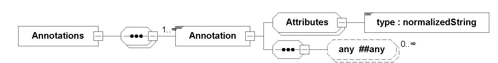
Each Annotation element contains a required type attribute, which contains the namespace for that annotation.
The content of the Annotation element can be arbitrary XML data, and can make use of XML namespaces and XML schemas for combined validation where appropriate.
The namespace mechanism for the type attribute is based on reverse domain notation:
The originator of a specification for additional data specifies a domain name under their control as the namespace for the additional data, in order to avoid conflicts due to name collisions.
All namespaces under both the org.modelica and org.fmi-standard domains are reserved for use in future layered standards.
[For example, extensions defined by the Modelica Association might make use of the org.modelica.fmi namespace.
This could lead to annotations with a type attribute of org.modelica.fmi.something, and/or extra files under the extra/org.modelica.ssp.something sub-directory.]
Annotations are intended to allow structured extensions of the FMI XML files, without creating conflicting extensions, or leaving ambiguities in interpretation. All annotations may safely be ignored by implementations that just implement the base FMI standard.
2.4.1. Model Description
Figure 9 shows the root element fmiModelDescription.
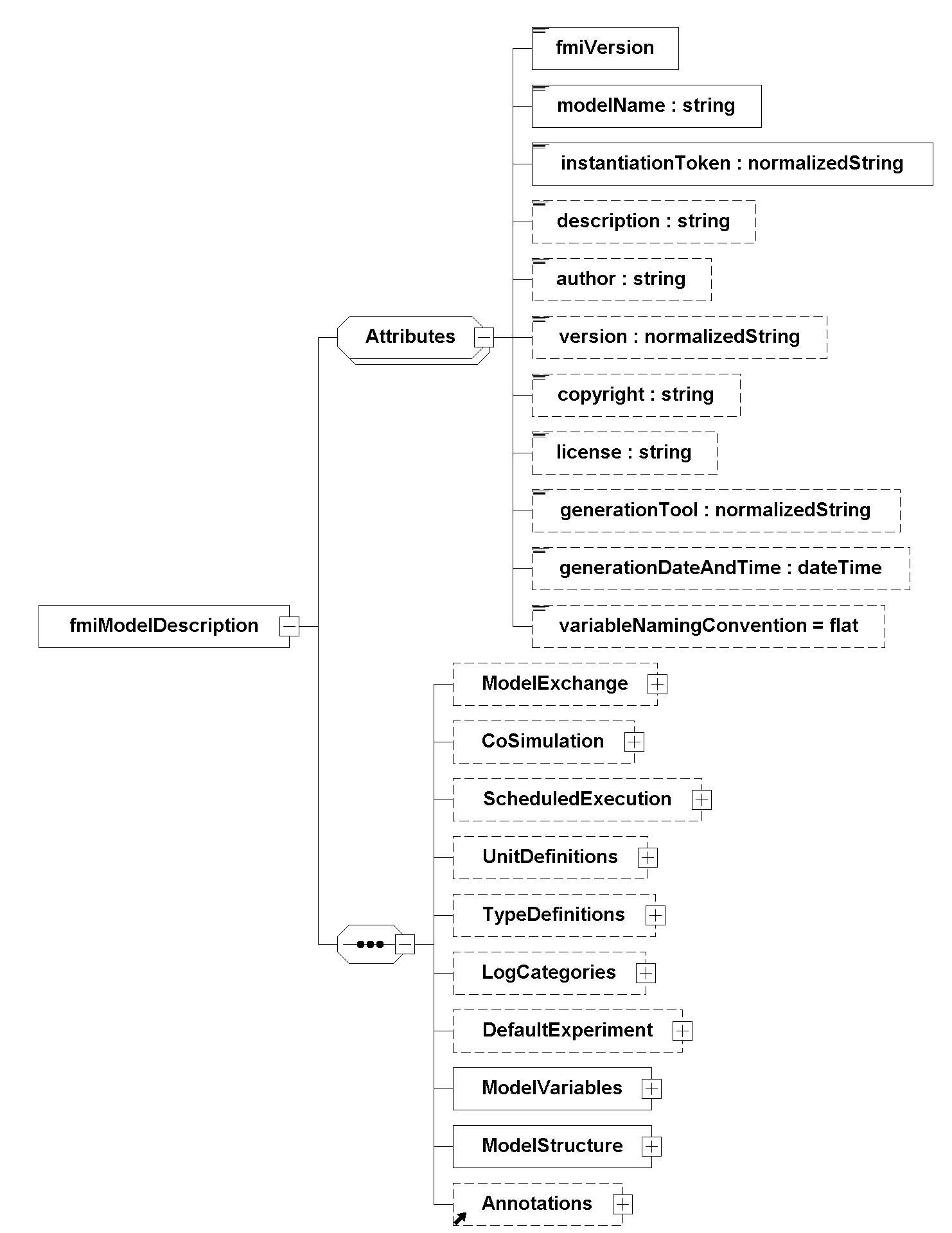
fmiModelDescription element.[If an optional element is present and defines a list (such as <UnitDefinitions>), the list must have at least one element (such as <Unit>).]
| Element | Description |
|---|---|
|
If present, the FMU is based on FMI for Model Exchange (Section 3). |
|
If present, the FMU is based on FMI for Co-Simulation (Section 4). |
|
If present, the FMU is based on FMI for Scheduled Execution (Section 5). |
|
A list of unit and display unit definitions [for example, used to convert display units into the units used in the model equations].
These definitions are used in the XML element |
|
A list of type definitions that are utilized in |
|
A list of log categories that can be set to define the log information that is supported from the FMU. |
|
Default settings for the importer algorithms, such as stop time and relative tolerance. |
A list of all variables of the FMU that are accessible via the FMU functions. |
|
Defines the structure of the model.
Especially, the ordered lists of |
|
Optional annotations for the top-level element. |
At least one element of <ModelExchange>, <CoSimulation> or <ScheduledExecution> must be present to identify the type of the FMU.
The details of these elements are defined in Section 3.4, Section 4.4 or Section 5.4.
How to support multiple interface types within one FMU, see Section 2.5.2.
The XML attributes of <fmiModelDescription> are:
| Attribute | Description |
|---|---|
|
Version of FMI the XML file complies with.
The value for this version is [During development prototype FMU implementations can indicate compliance with a certain development version based on the tags available at https://github.com/modelica/fmi-standard/tags.
For example the value for the FMI 3.0 Alpha 2 release is |
|
The name of the model as used in the modeling environment that generated the XML file, such as |
|
The |
|
Optional string with a brief description of the model. |
|
Optional string with the name of the model author. |
|
Optional version of the model [for example |
|
Optional information on the intellectual property copyright for this FMU [for example |
|
Optional information on the intellectual property licensing for this FMU. |
|
Optional name of the tool that generated the XML file. |
|
Optional date and time when the XML file was generated.
The format is a subset of |
Defines whether the variable names in |
2.4.2. Attributes and Capability Flags
The elements <ModelExchange>, <CoSimulation> and <ScheduledExecution> contain attributes, some representing capability flags, describing which optional functionalities the FMU supports.
Note that future FMI minor releases may add additional capability flags for optional features. Importers must be prepared to ignore unknown capability flags. Exporters must not generate capability flags without an XML namespace, unless specified by this standard or any later release of this standard.
The following table contains attributes and capability flags common to all three interface types.
For all Boolean attributes the default is false.
| Attribute | Description |
|---|---|
|
Short class name according to C syntax, for example, |
|
If |
|
If |
|
If |
|
If |
|
If |
|
If |
|
If |
|
If |
2.4.3. Physical Units
This section describes how units for variables can be defined. These descriptions allow automatic unit checks and value conversion in the importer to bridge the gap between FMUs from different simulation domains. The FMI unit descriptions are more secure than using humanly readable unit strings only, because all units can be defined as combinations of the seven SI base units.
Element <fmiModelDescription><UnitDefinitions> is defined as:
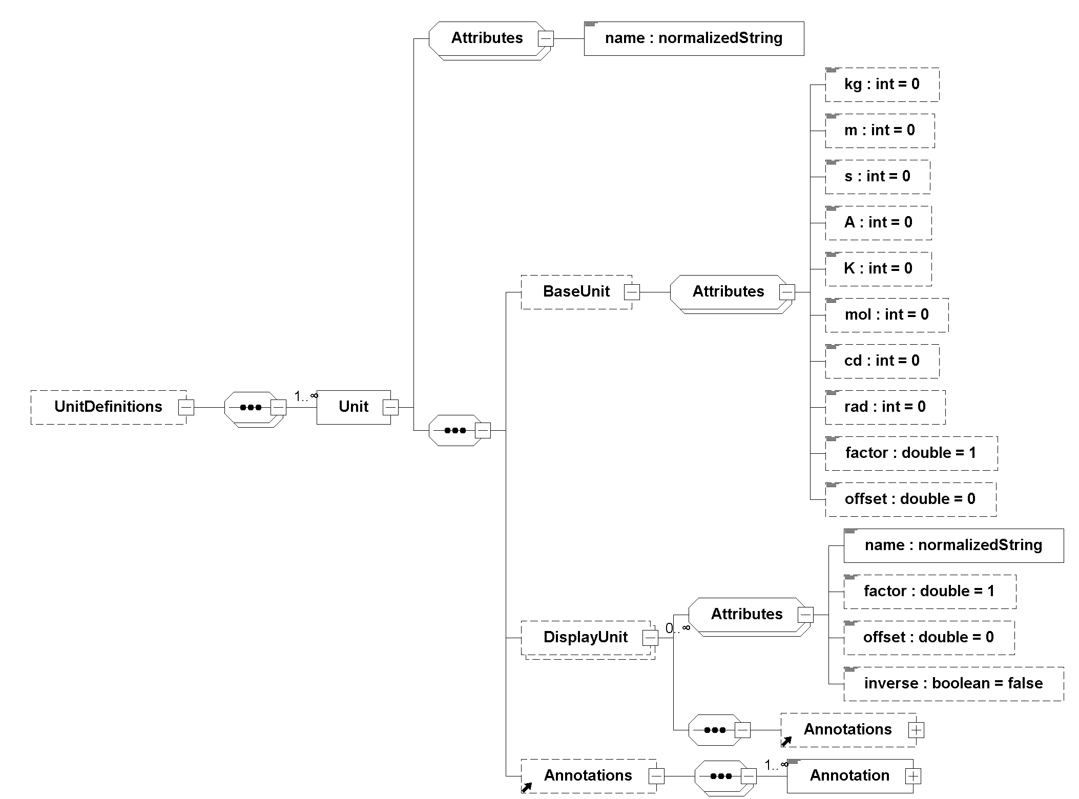
UnitDefinitions element.Units are referenced via its unique attribute name by the attribute unit and displayUnit of variable types and variables.
The name of a Unit must be unique with respect to all other <Unit> elements.
If a variable is associated with a Unit, the value passed to fmi3Set{VariableType} (resp. retrieved with fmi3Get{VariableType}) has this unit.
[The purpose of the name is to uniquely identify a unit and, for example, use it to display the unit in menus or in plots.
Since there is no standard to represent units in strings, and there are different ways how this is performed in different tools, no specific format for the string representation of the unit is required.]
The Unit definition consists of the exponents of the seven SI base units kg, m, s, A, K, mol, cd, the exponent of the SI derived unit rad, and optionally a factor and an offset.
[The additional rad base unit helps to handle the often occurring quantities in technical systems that depend on an angle.]
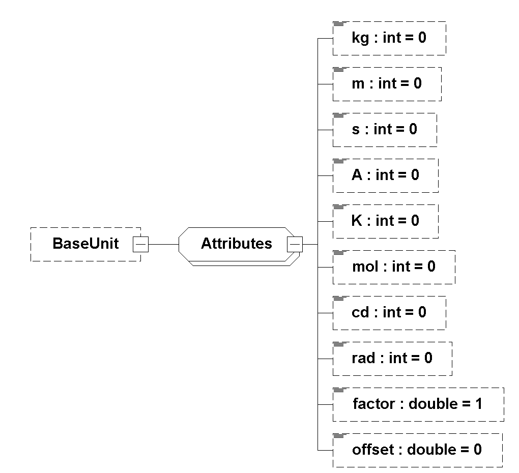
BaseUnit element.A value \(v_{\mathit{unit}}\) in Unit is converted to the base unit \(v_{\mathit{base}}\) by the equation
where factor and offset are attributes of the <BaseUnit>, and relativeQuantity an attribute of the TypeDefinition of a variable.
[For example, if \({p_{\mathit{bar}}}\) is a pressure value in unit bar, and \({p_{\mathit{Pa}}}\) is the pressure value in <BaseUnit>, then
and therefore, factor = 1.0e5 and offset = 0.0.
In the following table several unit examples are given.
Note that if in column exponents the definition \(\frac{kg \cdot m^2}{s^2}\) is present, then the attributes of <BaseUnit> are kg=1, m=2, s=-2.
Quantity |
Unit.name (examples) |
Unit.BaseUnit |
||
|---|---|---|---|---|
exponents |
factor |
offset |
||
Torque |
|
\({kg \cdot m^2 / s^2}\) |
|
|
Energy |
|
\({kg \cdot m^2 / s^2}\) |
|
|
Pressure |
|
\({\frac{kg}{m \cdot s^2}}\) |
|
|
Angle |
|
|
|
|
Angular velocity |
|
|
|
|
Angular velocity |
|
|
|
|
Frequency |
|
|
|
|
Temperature |
|
|
|
|
Percent by length |
|
|
|
|
Parts per million |
|
|
|
|
Length |
|
|
|
|
Length |
|
|
|
|
Note that Hz is typically used as Unit.name for a frequency quantity, but it can also be used as <DisplayUnit> for an angular velocity quantity (since revolution/s).
The <BaseUnit> definitions can be utilized for different purposes (the following application examples are optional and a tool may also completely ignore the Unit definitions):
- Unit check when connecting variables of different FMUs
-
When only one of
inputv2andoutputv1, connected with equationv2 = v1, defines a<BaseUnit>element,fmi3Get{VariableType}must be used to get the value ofv1to then set it withfmi3Set{VariableType}forv2.When two variables v1 and v2 are connected and for both of them
<BaseUnit>elements are defined, then they must have identical exponents of their<BaseUnit>. Iffactorandoffsetare also identical, again the connection equationv2 = v1holds. Iffactorandoffsetare not identical, the tool may either trigger an error or, if supported, perform a conversion; in other words, use the connection equation (in this case therelativeQuantityof the<TypeDefinition>, see below, has to be taken into account in order to determine whetheroffsetshall or shall not be utilized):factor(v1) * v1 + (if relativeQuantity(v1) then 0 else offset(v1)) = factor(v2) * v2 + (if relativeQuantity(v2) then 0 else offset(v2))
whererelativeQuantity(v1) = relativeQuantity(v2)is required.As a result, wrong connections can be detected (for example, connecting a force with an angle-based variable would trigger an error) and conversions between, say, US and SI units can be either automatically performed or, if not supported, an error is triggered as well.
This approach is not satisfactory for variables belonging to different quantities that have, however, the same
<BaseUnit>, such as quantitiesEnergyandTorque, orAngularVelocityandFrequency. To handle such cases, quantity definitions have to be taken into account (see<TypeDefinitions>) and quantity names need to be standardized.This approach allows a general treatment of units, without being forced to standardize the grammar and allowed values for units (for example, in FMI 1.0, a unit could be defined as
N.min one FMU and asN*min another FMU, and a tool would have to reject a connection, since the units are not identical. In FMI 2.0, the connection would be accepted, provided both elements have the same<BaseUnit>definition). - Dimensional analysis of equations
-
In order to check the validity of equations in a modeling language, the defined units can be used for dimensional analysis, by using the
<BaseUnit>definition of the respective unit. For this purpose, the<BaseUnit>radhas to be treated as1. Example:\[\begin{align*} J \cdot \alpha = \tau \rightarrow [kg.m^2]*[rad/s^2] = [kg.m^2/s^2] & \quad \text{// o.k. ("rad" is treated as "1")} \\ J \cdot \alpha = f \rightarrow [kg.m^2]*[rad/s^2] = [kg.m/s^2] & \quad \text{// error, since dimensions do not agree} \end{align*}\] - Unit propagation
-
If unit definitions are missing for variables, they might be deduced from the equations where the variables are used. If no unit computation is needed,
radis propagated. If a unit computation is needed and one of the involved units hasradas a<BaseUnit>, then unit propagation is not possible. Examples:-
a = b + c, and
Unitof c is provided, but notUnitof a and b:
The Unit definition ofc(in other words,Unit.name,<BaseUnit>,<DisplayUnit>) is also used foraandb. For example, if BaseUnit(c) =rad/s, then BaseUnit(a) = BaseUnit(b) =rad/s. -
a = b*c, and
Unitof a and of c is provided, but notUnitof b:
Ifradis either part of the<BaseUnit>ofaand/or ofc, then the<BaseUnit>ofbcannot be deduced (otherwise it can be deduced). Example: IfBaseUnit(a) = kg.m/s2andBaseUnit(c) = m/s2, then theBaseUnit(b)can be deduced to bekg. In such a caseUnit.nameof b cannot be deduced from theUnit.nameofaandc, and a tool would typically construct theUnit.nameofbfrom the deduced<BaseUnit>.]
-
A <Unit> can contain any number of <DisplayUnit> elements.
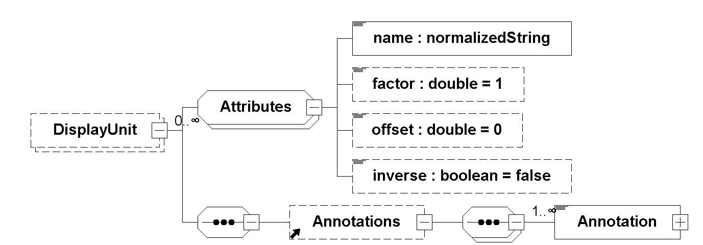
A <DisplayUnit> is defined by name, factor, offset, and inverse.
The attribute name must be unique with respect to all other names of the <DisplayUnit> definitions of the same Unit.
[Different Unit elements may have the same <DisplayUnit> names].
inverse = true is only allowed if offset = 0.
[Reason: no use case is known for the combination of inverse and offset, which would also be more complicated.]
A value \(v_{\mathit{unit}}\) in Unit is converted to a value \(v_{\mathit{display}}\) in DisplayUnit by the equation:
[offset is needed for temperature units like F (Fahrenheit), inverse for inverse display units like mpg (miles per gallon) or S (Siemens).
For example, if \({T_K}\) is the temperature value of Unit.name (in K) and \({T_F}\) is the temperature value of <DisplayUnit> (in °F), then
and therefore, factor = 1.8 (=9/5) and offset = -459.67 (= 32 - 273.15*9/5).
Both the DisplayUnit.name definitions as well as the Unit.name definitions are used in the variable elements.
Example of a definition:
<UnitDefinitions>
  <Unit name="rad/s">
    <BaseUnit s="-1" rad="1"/>
    <DisplayUnit name="deg/s" factor="57.29577951308232"/>
    <DisplayUnit name="rev/min" factor="9.549296585513721"/>
  </Unit>
  <Unit name="bar">
    <BaseUnit kg="1" m="-1" s="-2" factor="1e5" offset="0"/>
  </Unit>
  <Unit name="L/100km">
    <BaseUnit m="2" factor="1e-8"/>
    <DisplayUnit name="mpg" inverse="true" factor="235.214583"/>
  </Unit>
  <Unit name="Re">
    <BaseUnit/> <!-- unit="1" -->
                <!-- (dimensionless, all exponents of BaseUnit are zero) -->
  </Unit>
  <Unit name="Euro/PersonYear"/>  <!-- no mapping to BaseUnit defined -->
</UnitDefinitions>
]
2.4.4. Variable Types
Element <fmiModelDescription><TypeDefinitions> is defined as:
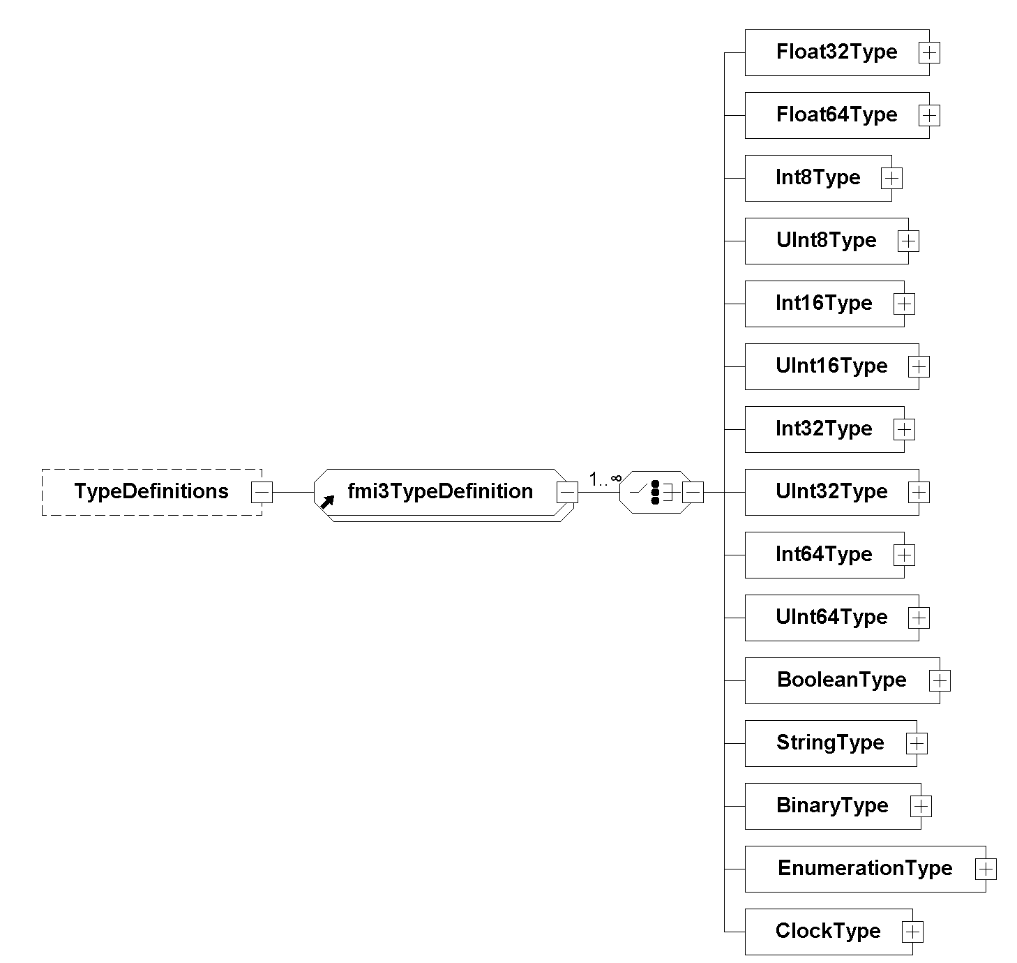
This element consists of a set of <TypeDefinition> elements according to schema fmi3TypeDefinition in file fmi3Type.xsd.
Each variable type has its own set of attributes. Figure 14, Figure 15, Figure 16, Figure 17, Figure 18, and Figure 19 are representative examples.
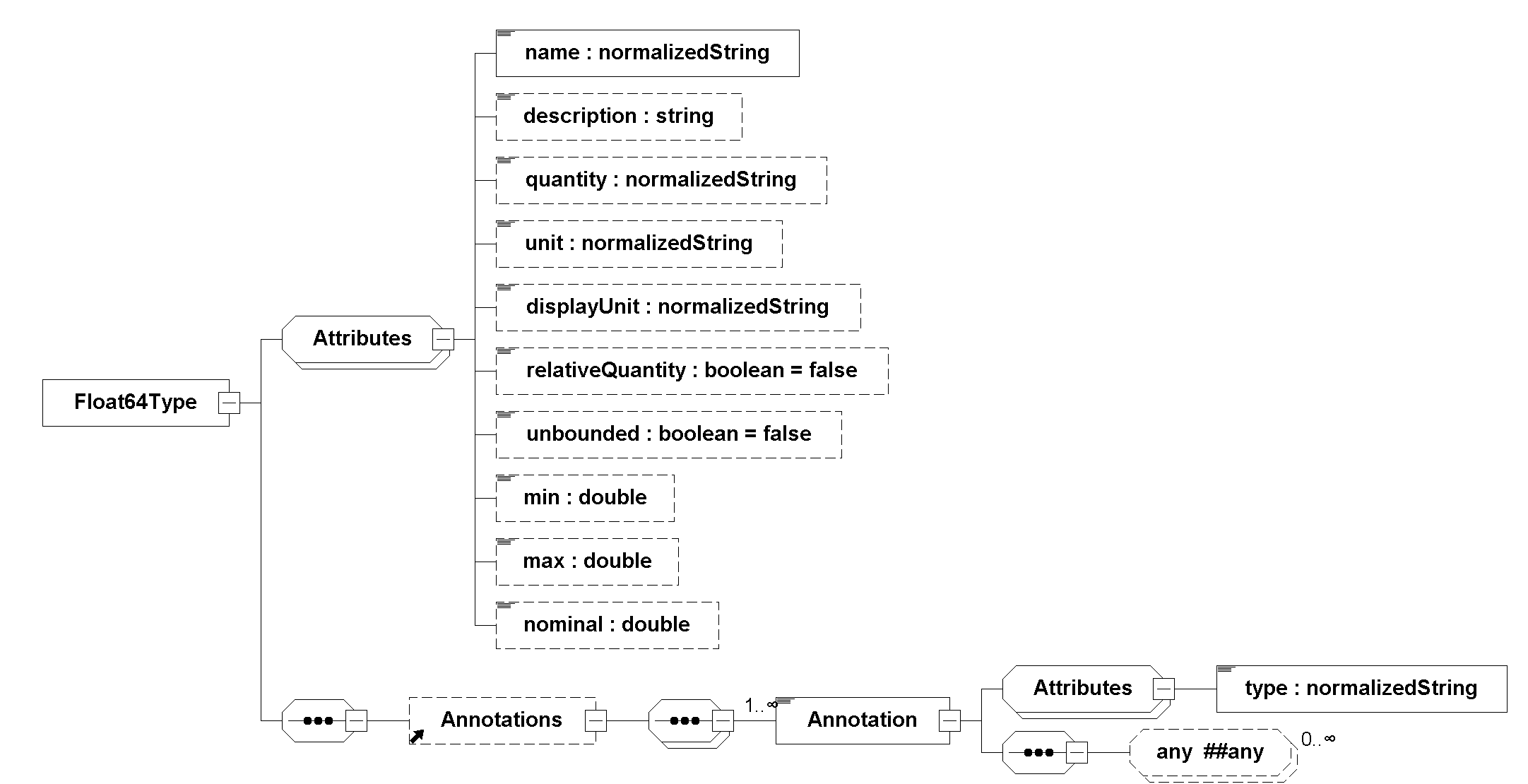
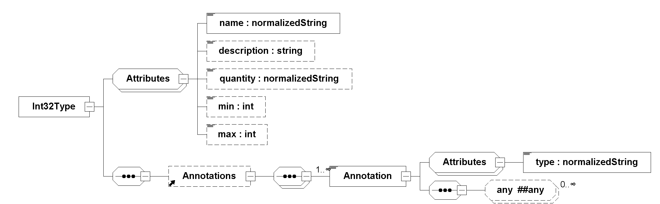
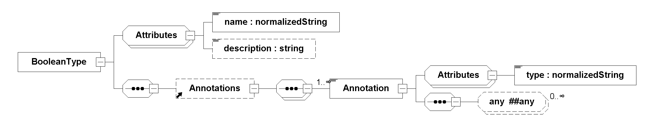
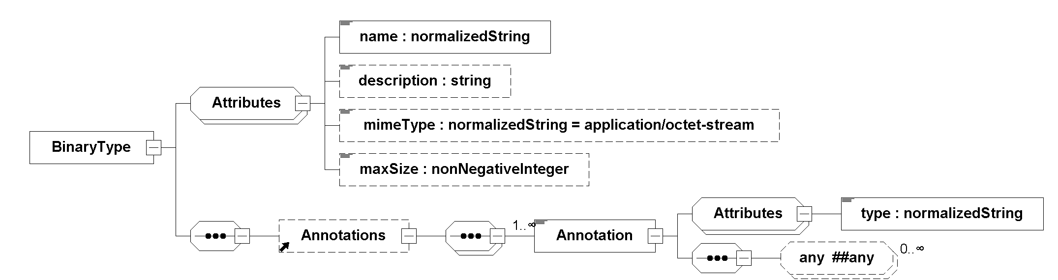
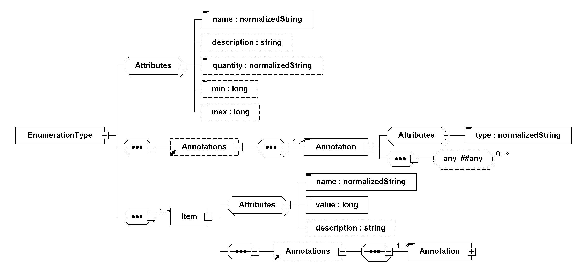
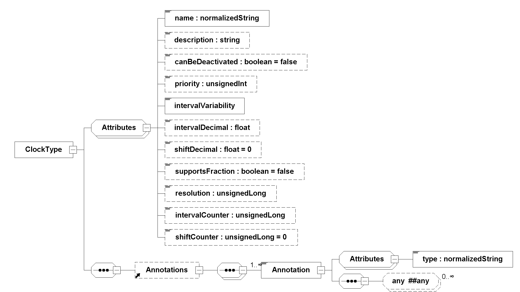
The <TypeDefinition> elements are referred to in variable elements to declare their type.
[The alternative would be to define a type per variable.
However, this would lead to a situation where, e.g., the definition of a Torque type would have to be repeated over and over.]
The attributes and elements have the following meaning:
| Attribute or Element | Description |
|---|---|
|
The unique name of the variable type referenced using the attribute |
|
An optional description string describing the meaning of the variable type. |
|
Physical quantity of the variable.
[For example, |
|
Unit of the variable referencing to a |
|
Default display unit of the variable referencing to a |
|
Indicates the type of data passed as a binary.
Defaults to |
|
Indicates the maximum size (bytes) of the data passed as a binary. |
|
If this attribute is |
|
Minimum value of variable (variable value \(\geq\) |
|
Maximum value of variable (variable value \(\leq\) |
|
Nominal value of variable.
If not defined and no other information about the nominal value is available, then |
|
If |
|
An |
Attributes for |
|
|
|
|
This attribute is mandatory for input |
|
The attribute |
The values of the following float and integer attributes refer to the unit of the |
|
|
This attribute defines the time interval \(T_{\mathit{interval}}\) between consecutive Clock ticks.
This value must be greater than 0.0.
This attribute is required if Clock type is |
|
This attribute defines the delay of the first clock activation relative to \(t_{\mathit{start}}\) ( |
|
This attribute defines, if the functions |
|
Instead of defining clock timing using floating point numbers, FMI allows the definition of rational numbers using |
|
This attribute defines (together with \(T_{\mathit{interval}} = \)
|
|
This value defines (together with \(T_{\mathit{shift}} = \) This attribute requires that |
2.4.5. Log Categories
Element <fmiModelDescription><LogCategories> is defined as:
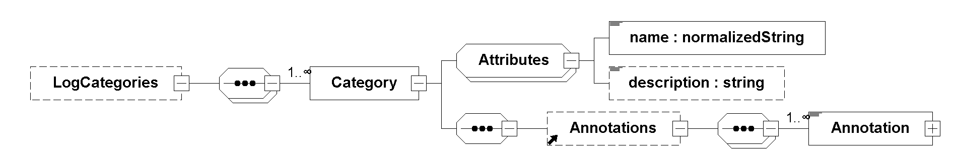
<LogCategories> defines an unordered set of category strings that classify output of the callback function logMessage.
The importer may use the function fmi3SetDebugLogging to control for which <LogCategories> the callback function logMessage is allowed to be called.
The name attribute of <Category> must be unique with respect to all other elements of the <LogCategories> list.
Table 16 shows the standardized values for name of <Category>.
These names should be used if a tool supports the corresponding log category.
If an FMU supports one of these log categories, then an element <Category> with this name must be added to <LogCategories>.
Any other FMU specific <LogCategories> may be defined.
| Category | Description |
|---|---|
|
Log all events (during initialization and simulation). |
|
Log the solution of linear systems of equations if the solution is singular (and the tool picked one solution of the infinitely many solutions). |
|
Log the solution of nonlinear systems of equations. |
|
Log the dynamic selection of states. |
|
Log messages when returning |
|
Log messages when returning |
|
Log messages when returning |
|
Log messages when returning |
The optional attribute description shall contain a description of the respective log category.
[Typically, this string can be shown by a tool if more details for a log category are presented.
This approach to define <LogCategories> has the following advantages:
-
An importer may present the possible log categories in a menu and the user can select the desired one.
-
The log output is drastically reduced, because via
fmi3SetDebugLoggingthe categories are set that shall be logged and therefore the FMU will print only the messages with the corresponding categories to thelogMessagefunction.
Note that since element <LogCategories> is optional, an FMU does not need to expose its log categories.]
2.4.6. Default Experiment
Element <fmiModelDescription><DefaultExperiment> is defined as:
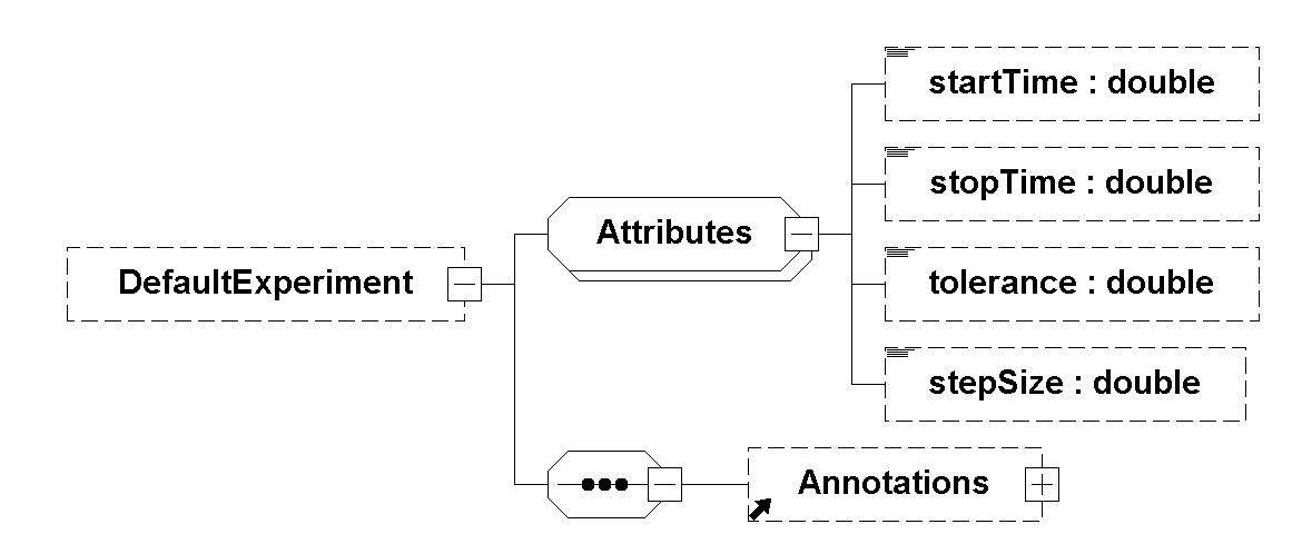
<DefaultExperiment> consists of the optional default start time, stop time, relative tolerance, and step size for a simulation run.
A tool may ignore this information.
[However, it is convenient for a user that startTime, stopTime, tolerance and stepSize have already a meaningful default value for the model at hand.]
Furthermore, for Co-Simulation FMUs the stepSize defines the preferred communicationStepSize.
startTime, stopTime and stepSize refer to the unit of the independent variable.
2.4.7. Model Variables
2.4.7.1. Static information
The element of <fmiModelDescription><ModelVariables> is the central part of the modelDescription.xml.
It provides the static information of all exposed variables and is defined as follows:
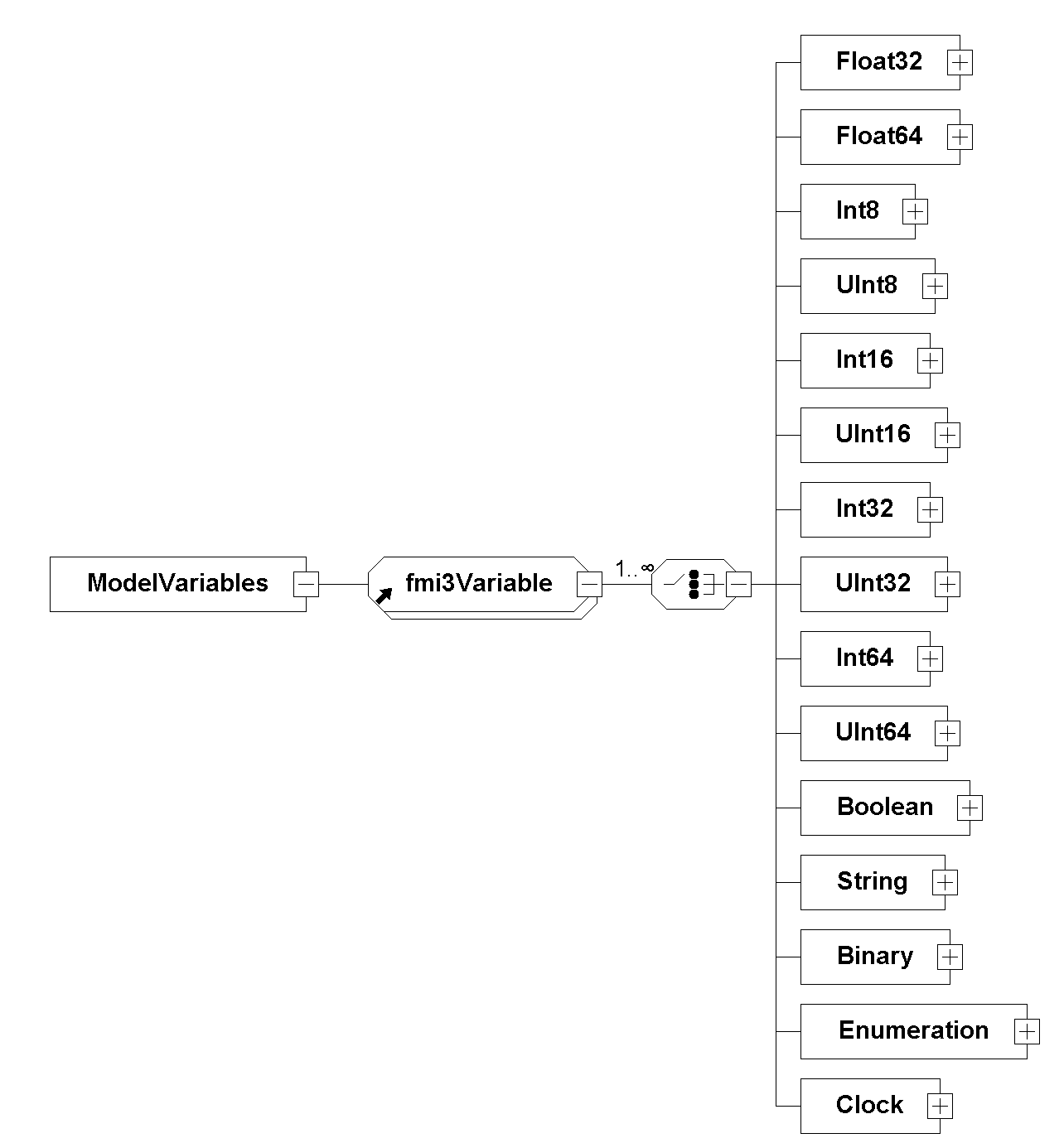
The <ModelVariables> element consists of an arbitrary number of <fmi3Variable> elements (see Figure 22).
<fmi3Variable> elements represent scalars or arrays of an arbitrary (but fixed) number of dimensions for variables of different types, like single-precision floating point, string or binary.
The schema definition is present in a separate file fmi3Variable.xsd.
2.4.7.2. Array variables and structural parameters
Except for Clocks, variable elements can represent an array variable.
Variable elements representing array variables must contain at least one <Dimension> element.
Each <Dimension> element specifies the size of one dimension of the array:
-
If the
startattribute of the<Dimension>element is present, it defines a constant unsigned 64-bit integer size for this dimension. Thevariabilityof the dimension size isconstantin this case. -
If the
valueReferenceattribute of the<Dimension>element is present, it defines the size of this dimension to be the value of the variable with the value reference given by thevalueReferenceattribute. The referenced variable must be a variable of type<UInt64>, and must either be a constant (i.e. withvariability=constant) or astructural parameter(i.e. withcausality=structuralParameter). Thevariabilityof the dimension size is in this case thevariabilityof the referenced variable. Astructural parametermust be a variable of type<UInt64>only if it is referenced in<Dimension>.
These two options are mutually exclusive, i.e., for each <Dimension> element either a start attribute or a valueReference attribute can be supplied, but not both.
However different <Dimension> sizes for the same variable may be specified using different mechanisms by having different variability attributes.
All initial dimension sizes (defined by start values either directly or indirectly in the <fmiModelDescription>) must be positive integers (i.e. not zero), so that no dimension is initially vanished.
[This allows importers to ignore structural parameters because their start values reflect the internal default settings of structural parameters.
If we allowed 0 dimension sizes for initial values, tools that do not even care about changing dimension sizes would need to be able to handle vanishing arrays.]
[Example:
The variable V is a floating point vector parameter.
The length of the vector depends on the structural parameter len, connected via the valueReference = "100".
The default length of the vector is 7.
This length can be changed in Configuration Mode because the variability of the structural parameter len is fixed.
The values of V can be changed whenever tunable parameters can be changed.
<UInt64 name="len" valueReference="100" causality="structuralParameter"
  variability="fixed" start="7"/>
<Float32 name="V" valueReference="1" causality="parameter" variability="tunable"
  start="0.1 -0.2 0.3 -0.4 0.5 -0.6 0.7">
  <Dimension valueReference="100"/>
</Float32>
]
Changes to dimension sizes are constrained by the min/max attributes of the referenced structural parameters, which can be any non-negative integer, including zero.
Specifying a minimum size of zero on a structural parameter allows any related dimension sizes to be changed to zero in Configuration Mode or Reconfiguration Mode, thus causing the respective array size to go to zero, which leaves the respective array variable without any active elements.
The actual dimension sizes of arrays are also constrained by the importer, due to memory and addressing constraints:
Since the API functions to access variables and their values are constrained to size_t individual elements, platforms with addresses of less than 64-bit width will not be able to access elements beyond their addressing limits, neither will they be able to allocate enough memory or address space to represent such arrays.
For these reasons implementations must take platform-specific constraints into account when changing dimension sizes, and must be prepared to handle the inability of the FMU to adjust to the desired sizes during Configuration Mode or Reconfiguration Mode.
Changing any dimension of a variable in Configuration Mode or Reconfiguration Mode invalidates the variable’s current value (including its start value).
Changing one structural parameter might affect dimension sizes of several variables.
2.4.7.3. Alias variables
A variable can have any number of <Alias> elements that define a variable alias.
Each variable alias has a required attribute name whose value must be unique among all variables and variable aliases, and an optional attribute description.
Variable aliases of floating point variables may additionally have a displayUnit that follows the same rules as for variables.
[ Example:
 <Float64 name="engine.torque" valueReference="1" unit="N.m">
   <Alias name="engine.torqueLbfFt" description="Engine torque in pound-foot"
     displayUnit="lbf.ft"/>
 </Float64>
]
2.4.7.4. Variable Attributes
The common attributes of variables are shown in Figure 23.
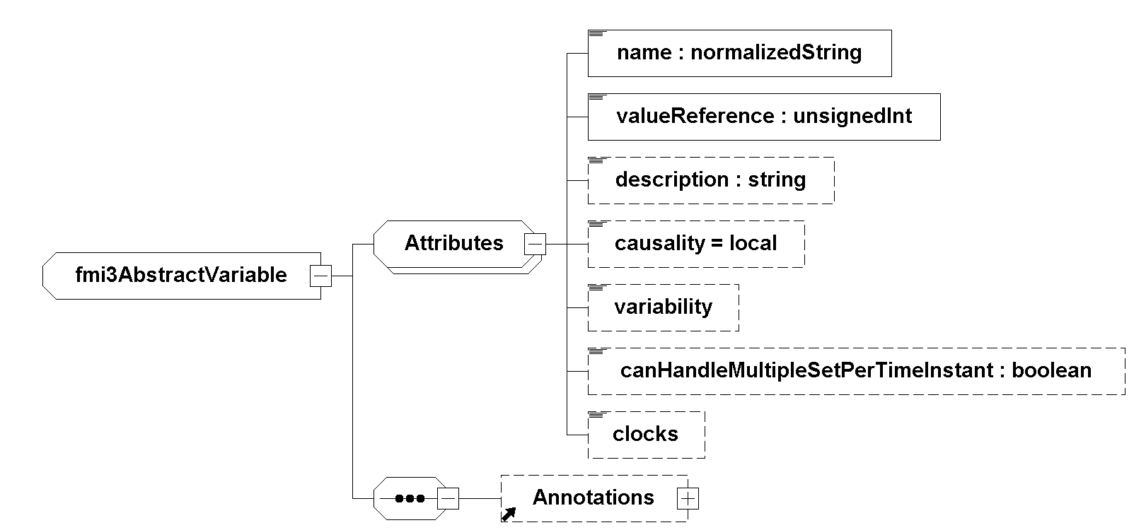
| Attribute | Description |
|---|---|
|
The unique name of the variable. This attribute may follow a defined naming convention. |
|
A handle of the variable to identify the variable value in the C-API functions and for references within the |
|
An optional description string describing the meaning of the variable. |
|
Enumeration that defines the causality of the variable.
Allowed combinations of Values of this enumeration are:
Setting of local variables:
Local variable values must not be used as input to another model or FMU.
|
|
Enumeration that defines the time dependency of the variable, in other words, it defines the time instants when a variable may be changed by the importer or may change its value due to FMU internal computations, depending on their [For example, Allowed combinations of Values of this enumeration are:
The
For more explanations on value changes see Section 4.1.1. |
|
Only for variables with [This flag can be set to |
|
If this boolean attribute is This attribute is ignored in Model Exchange and Scheduled Execution.
Variables of type Clock must not have the |
|
If present, this variable is a
[For example, if |
|
If present, this variable is clocked.
The value of the attribute |
Table 18 shows the combinations of variability/causality settings that are allowed.
— (a) |
— (a) |
— (a) |
— (a) |
(7) |
(10) |
— (c) |
|
(16) |
(1) |
(3) |
— (d) |
— (e) |
(11) |
— (c) |
|
(17) |
(2) |
(4) |
— (d) |
— (e) |
(12) |
— (c) |
|
— (b) |
— (b) |
— (b) |
(5) |
(8) |
(13) |
— (c) |
|
— (b) |
— (b) |
— (b) |
(6) |
(9) |
(14) |
(15) |
|
[Discussion of the combinations that are not allowed:
| Explanation why this combination is not allowed | |
|---|---|
(a) |
The combinations |
(b) |
The combinations |
(c) |
For an |
(d) |
A |
(e) |
A |
Discussion of the combinations that are allowed:
| Setting | Example | |
|---|---|---|
(1) |
||
(2) |
||
(3) |
Non- |
|
(4) |
|
|
(5) |
||
(6) |
|
|
(7) |
Variable where the value never changes and that can be used in another model. |
|
(8) |
|
|
(9) |
|
|
(10) |
Variable that never changes its value. Cannot be used in another model. |
|
(11) |
Local variable that depends on |
|
(12) |
Local variable that depends on |
|
(13) |
|
|
(14) |
|
|
(15) |
All variables are a function of the continuous-time variable marked as |
|
(16) |
|
|
(17) |
|
How to treat tunable variables:
A parameter p is a variable that does not change its value during simulation, in other words, dp/dt = 0.
If the parameter p is changing, then Dirac impulses are introduced since dp/dt of a discontinuous constant variable p is a Dirac impulse.
Even if this Dirac impulse would be modeled correctly by the FMU, it would introduce unwanted vibrations.
Furthermore, in many cases the model equations are derived under the assumption of a constant value (like mass or capacity), and the model equations would be different if p would be time varying.
FMI for Model Exchange:
Therefore, "tuning a (structural) parameter" during simulation does not mean to "change the parameter online" during simulation.
Instead, this is a short hand notation for:
-
Stop the simulation at an event instant (usually, a step event, in other words, after a successful integration step).
-
Change the values of the
tunable(structural)parameters. Fortunablestructural parameters, the Reconfiguration Mode must be entered before and left afterwards. -
Compute all
parameters(and sizes of variables, states,derivatives, event indicators, …) that depend on thetunable(structural)parameters. -
Newly start the simulation using as initial values previously stored values and the new values of the
parameters.
Basically this means that a new simulation run is started from the previous FMU state with changed parameter values.
With this interpretation, changing parameters online is "clean", as long as these changes appear at an event instant.
FMI for Co-Simulation:
Changing of tunable parameters is allowed before an fmi3DoStep call (so, whenever an input can be set with fmi3Set{VariableType}) and before fmi3ExitInitializationMode is called (that is before and during Initialization Mode).
The FMU internally carries out event handling if necessary.
FMI for Scheduled Execution:
Changing of tunable parameters is allowed before an fmi3ActivateModelPartition call (so, whenever an input can be set with fmi3Set{VariableType}) and before fmi3ExitInitializationMode is called (that is before and during Initialization Mode).]
2.4.7.5. Type-specific properties
<ModelVariables> can be of different types, for example Float64, Int32, Boolean, Binary, Enumeration and Clock.
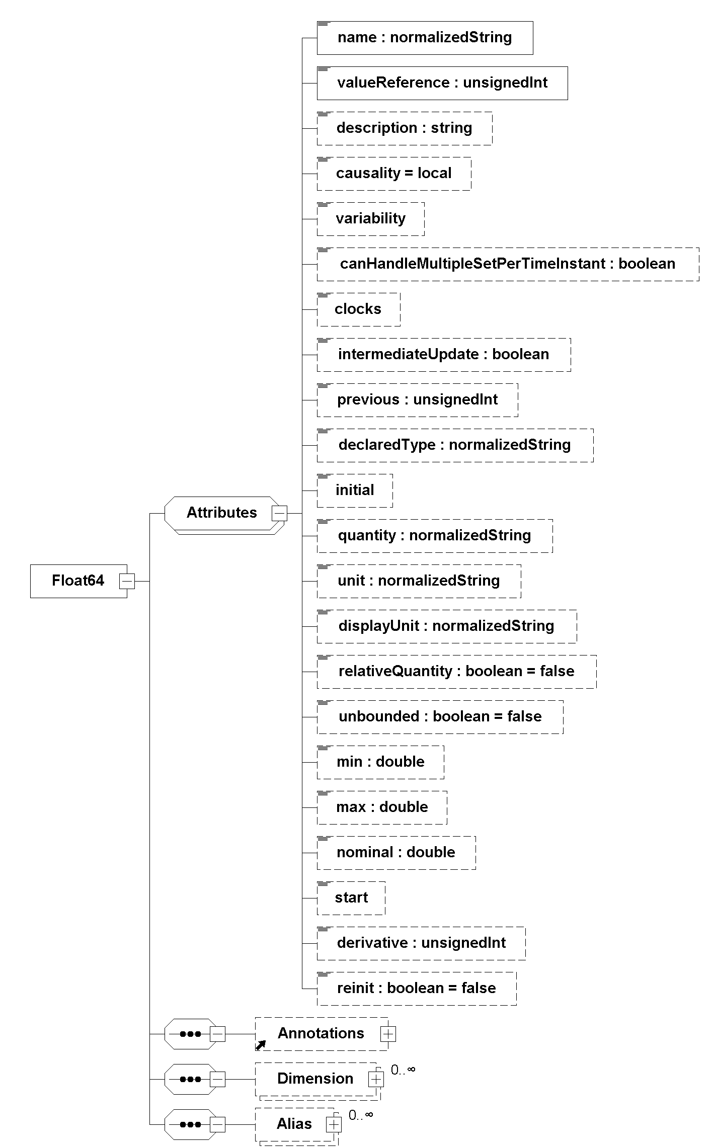
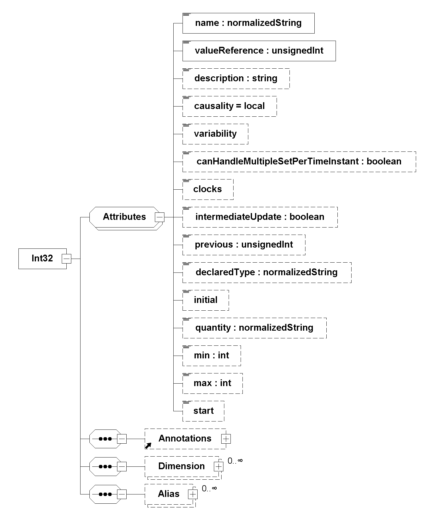
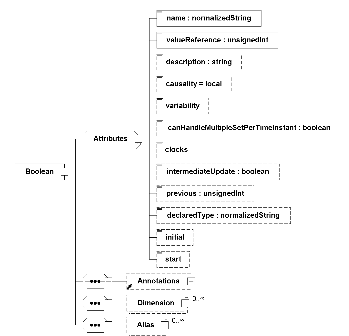
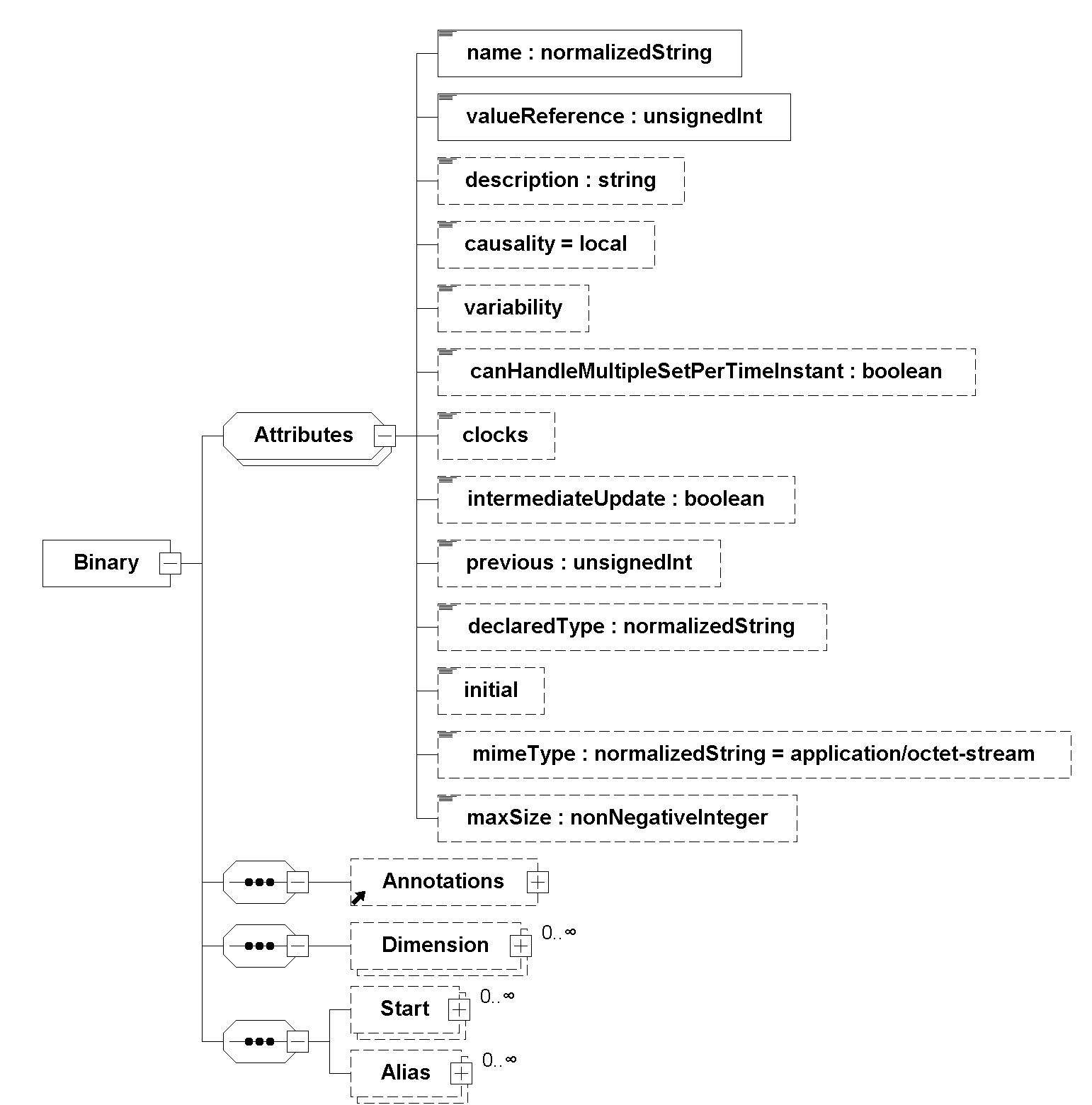
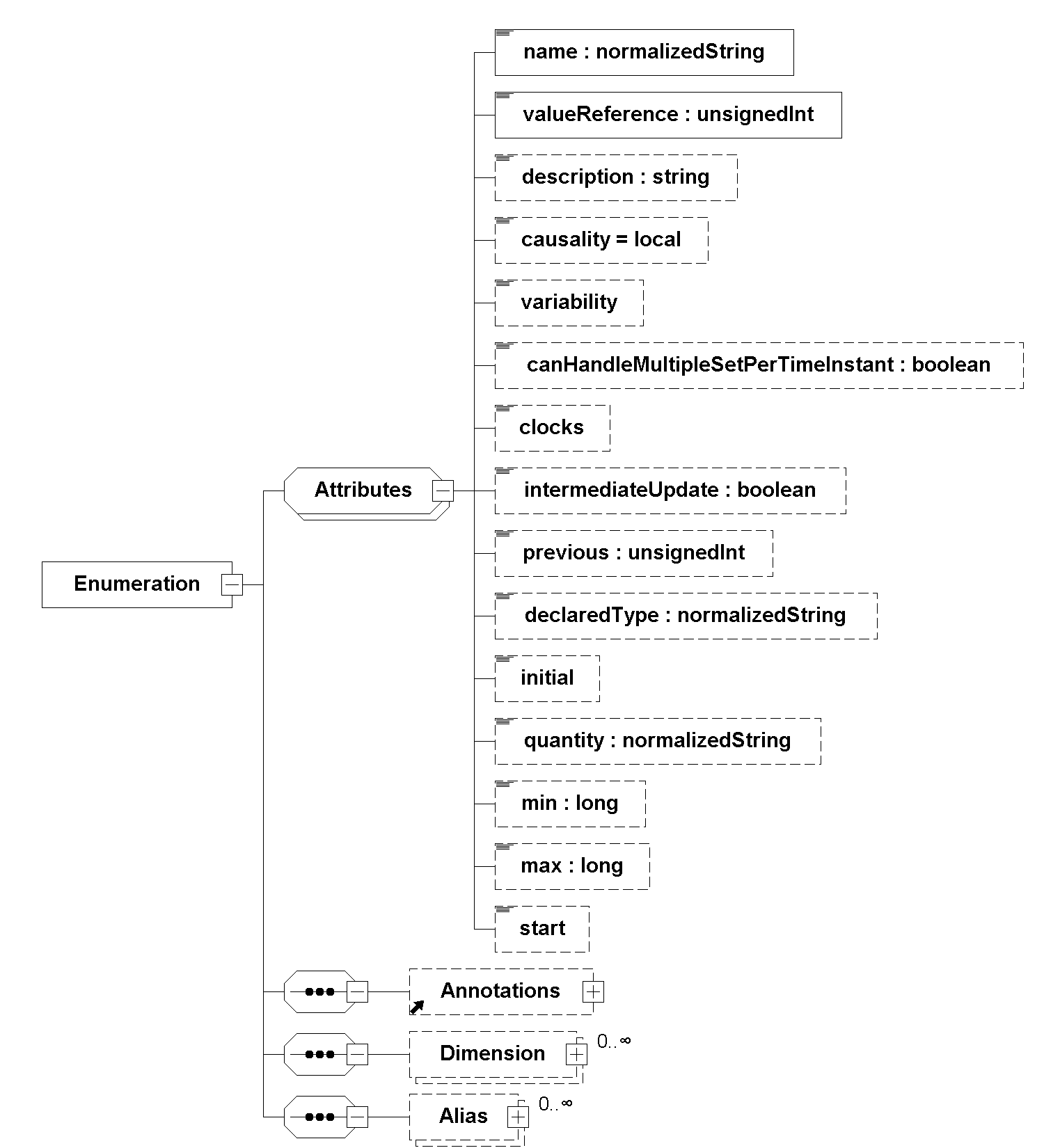
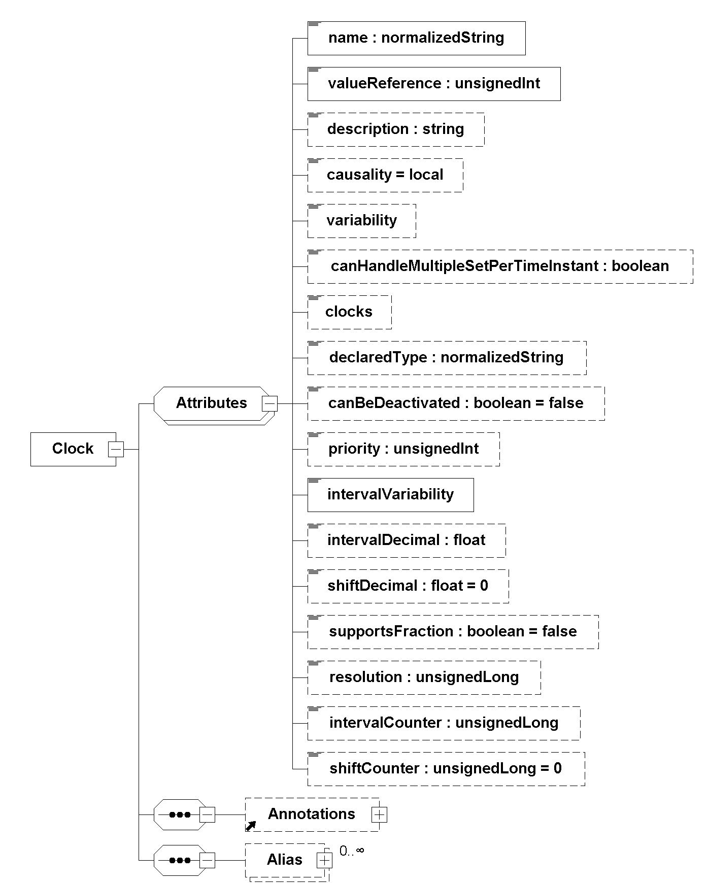
The attributes common to all variable types are defined in Table 15 and Table 17. Type specific attributes are listed in the following table.
| Attribute | Description |
|---|---|
|
If present, name of type defined with |
|
This attribute defines the unit of the variable by referencing a |
|
Default display unit of the variable referencing to a |
|
Enumeration that defines how the variable is initialized, i.e. if a For the variable with The attribute
Table 22 defines the allowed values for |
|
Initial or guess value of the variable.
During instantiation, the FMU initializes its variables with their The For variables of type [ Example: Start values of string array variable ] The interpretation of Variables with
|
|
If present, then the variable with this attribute is the derivative of the variable with value reference given in |
|
Only used in Model Exchange, ignored for the other interface types.
May only be present for a continuous-time state. |
If initial is not present in a type that can have that attribute, its value is defined by Table 22 based on the values of causality and variability (default underlined):
— |
— |
— |
— |
exact |
exact |
— |
|
exact |
exact |
calculated |
— |
— |
calculated |
— |
|
exact |
exact |
calculated |
— |
— |
calculated |
— |
|
— |
— |
— |
exact |
calculated |
calculated |
— |
|
— |
— |
— |
exact |
calculated |
calculated |
— |
|
2.4.7.5.1. Variable Naming Conventions
With attribute variableNamingConvention in <fmiModelDescription>, the convention is defined how the variable names have been constructed.
The importer may use this information to represent the names in a better way (for example, as a tree and not as a linear list).
In the following definitions, the Extended Backus-Naur Form (EBNF) is used:
=   production rule
[ ] optional
{ } repeat zero or more times
|   or
The names must be unique, non-empty strings.
The following conventions for scalar names are defined:
name = Unicode-char { Unicode-char } // identical to xs:normalizedString
Unicode-char = any Unicode character without carriage return (#xD),
line feed (#xA) nor tab (#x9)
Structured names are using "." as a separator between hierarchies.
A name consists of "_", letters and digits or may consist of any characters enclosed in single apostrophes.
A name may identify an array element on every hierarchical level using "[…]" to identify the respective array index.
If an array is a leaf node of the variable hierarchy then the array can also be represented as a single variable of type array.
A derivative of a variable is defined with der(name) for the first time derivative and der(name,N) for the N-th derivative.
Examples:
vehicle.engine.speed
resistor12.u
v_min
robot.axis.'motor #234'
der(pipe[3,4].T[14],2) // second time derivative of pipe[3,4].T[14]
The precise syntax is:
name            = identifier | "der(" identifier ["," unsignedInteger ] ")"
identifier      = B-name [ arrayIndices ] {"." B-name [ arrayIndices ] }
B-name          = nondigit { digit | nondigit } | Q-name
nondigit        = "pass:[_]" | letters "a" to "z" | letters "A" to "Z"
digit           = "0" | "1" | "2" | "3" | "4" | "5" | "6" | "7" | "8" | "9"
Q-name          = "'" ( Q-char | escape ) { Q-char | escape } "'"
Q-char          = nondigit | digit | "!" | "#" | "$" | "%" | "&" | "(" | ")" |
                                     "*" | "+" | "," | "-" | "." | "/" | ":" |
                                     ";" | "<" | ">" | "=" | "?" | "@" | "[" |
                                     "]" | "^" | "{" | "}" | "|" | "~" | " "
escape          = "\'" | "\"" | "\?" | "\\" | "\a" | "\b" |
                  "\f" | "\n" | "\r" | "\t" | "\v"
arrayIndices    = "[" unsignedInteger {"," unsignedInteger} "]"
unsignedInteger = digit { digit }
[This definition is identical to the syntax of an identifier in the Modelica Language Specification.]
Example:
vehicle
  transmission
    ratio
    outputSpeed
  engine
    inputSpeed
    temperature
is mapped to the following list of variable names:
vehicle.transmission.ratio
vehicle.transmission.outputSpeed
vehicle.engine.inputSpeed
vehicle.engine.temperature
It might be that not all elements of an array are present.
The variableNamingConvention structured does not define if arrays are 0-based or 1-based.
2.4.8. Model Structure
The structure of the model is defined in element <fmiModelDescription><ModelStructure>.
It defines the dependencies between variables.
The required part of the model structure for all FMI types defines the ordering of outputs in <Output> and unknowns during initialization in <InitialUnknown>.
A Model Exchange FMU must also expose all derivatives of continuous states in <ContinuousStateDerivative> and all event indicators in <EventIndicator>.
The optional part of the model structure defines in which way derivatives, outputs, and initial unknowns depend on inputs and/or parameters, and continuous-time states.
The listed dependencies declare the dependencies between whole (multi-dimensional-)variables and not individual elements of the variables.
[Dependencies of individual array elements can be retrieved during runtime using fmi3GetVariableDependencies.]
Figure 30 shows the definition of <ModelStructure>.
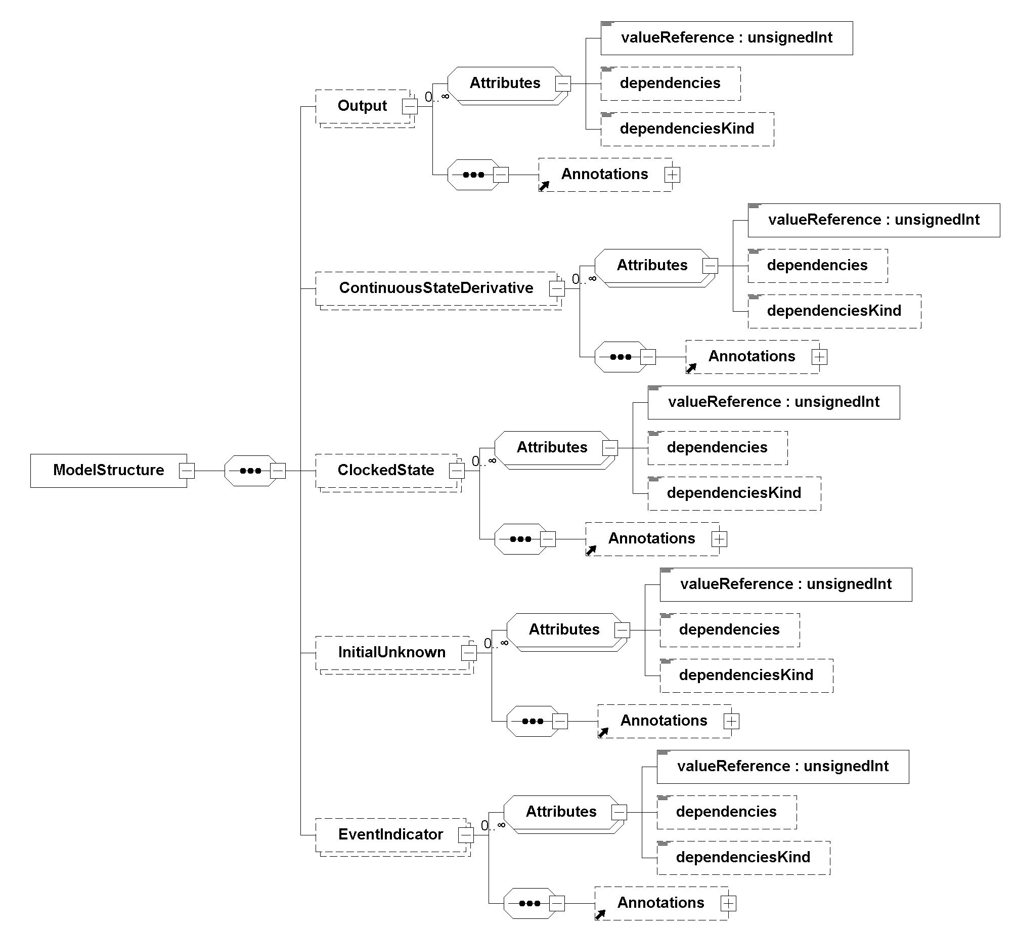
Note that attribute dependenciesKind for element <InitialUnknown> has less enumeration values as dependenciesKind in the other lists, as detailed in Table 23.
<ModelStructure> consists of the elements detailed in Table 23 (see also Figure 30; the symbols of the mathematical equations describing the dependencies are defined in Section 3.1):
| Element | Description |
|---|---|
|
Ordered list of all outputs, in other words, a list of value references where every corresponding variable must have |
|
Ordered list of value references of all derivatives of continuous states.
The order defined by this list defines the order of the elements for The corresponding continuous-time states are defined by attribute |
|
A |
|
Ordered list of all exposed unknowns in Initialization Mode. This list consists of all variables which:
The resulting list is not allowed to have duplicates (for example, if a state is also an \({\mathbf{v}_{\mathit{initialUnknowns}} := \mathbf{f}_{\mathit{init}}(\mathbf{u}_c, \mathbf{u}_d, t_{\mathit{start}}, \mathbf{v}_{\mathit{initial=exact}})}\) Since,
[Example: Assume an FMU is defined in the following way: \({(\mathbf{y}_{c+d}, \dot{\mathbf{x}}_c) := \mathbf{f}_{\mathit{init}}(\mathbf{x}_c, \mathbf{u}_{c+d}, t_{\mathit{start}}, \mathbf{p})}\) \({(\mathbf{y}_{c+d}, \dot{\mathbf{x}}_c) := \mathbf{f}_{\mathit{sim}}(\mathbf{x}_c, \mathbf{u}_{c+d}, t_i, \mathbf{p})}\) Therefore, the initial state \({\mathbf{x}_c(t_{\mathit{start}})}\) has |
|
An ordered list of value references where every referenced variable must be an event indicator.
The serialized (if value reference points to array variable) and concatenated values of the variables referenced by the attribute For Co-Simulation and Scheduled Execution, [The intention for connecting event indicators to variables via |
Elements <Output>, <ContinuousStateDerivative>, <ClockedState>, <InitialUnknown>, and <EventIndicator> have (partially) the following attributes:
| Attribute | Description |
|---|---|
|
The value reference of the unknown \({v_{\mathit{unknown}}}\). |
|
Optional attribute defining the algebraic dependencies as list of value references of the unknown \({\mathbf{v}_{\mathit{unknown}}}\) directly with respect to \({\mathbf{v}_{\mathit{known}}}\).
For a real valued unknown and a real valued known, if the known is not listed among the dependencies then the partial derivative of the unknown with respect to that known is identically zero.
If dependencies is not present, it must be assumed that the unknown depends on all knowns.
If dependencies is present as empty list, the unknown depends on none of the knowns.
Otherwise the unknown depends on the knowns defined by the given value references.
Knowns \({\mathbf{v}_{\mathit{known}}}\) in Initialization Mode (for elements
[The |
|
If
The following
The following
|
2.4.9. Terminals and Icons
Terminals define semantic groups of variables to ease connecting compatible signals on the system level.
This definition adds an additional layer to the interface description of the FMUs.
It does not change the causality of the variables (i.e. inputs and outputs), but enables the definition of physical and bus-like connectors that require special handling on the system level by the importer (e.g. flow variables and bus frames).
Icons define a graphical representation of an FMU and its terminals.
Both features are optional and may be defined in the separate XML file terminalsAndIcons/terminalsAndIcons.xml.
[The usage of a separate file enables backporting of this feature to previous FMI versions.]
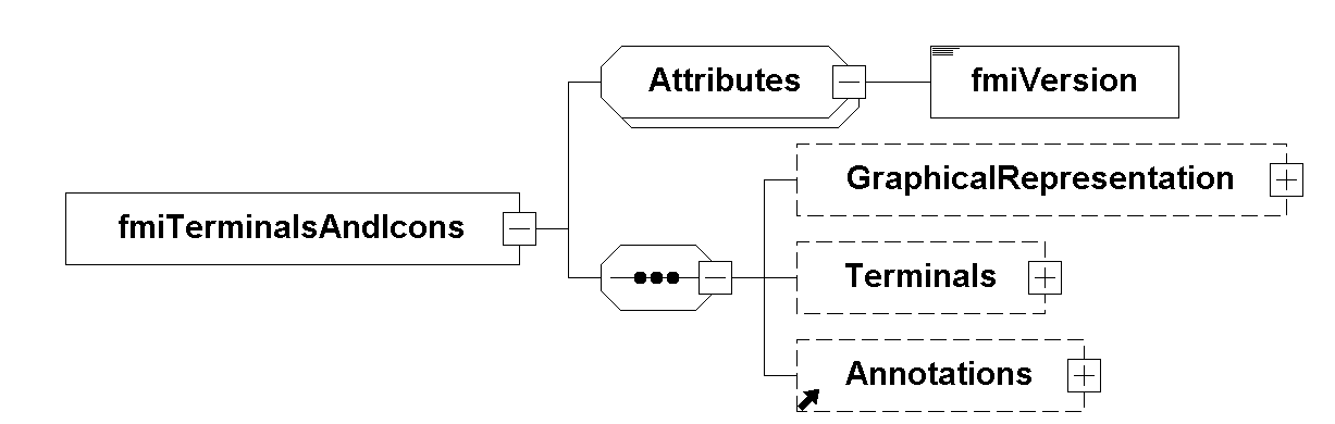
On the top level, the schema consists of the following elements (see Figure 31).
| Attribute or Element | Description |
|---|---|
|
This attribute declares the FMI version defining the XSD of the |
|
If present, contains information for importers of FMUs to draw graphical representations of the FMU in a system view. |
|
If present, this allows combining variables (e.g. inputs, outputs and parameters) into logical groups to ease connections on a system level and add semantic information required for system-level connections. |
2.4.9.1. Definition of a Graphical Representation
2.4.9.1.1. Overview
The graphical representation of the FMU and terminals are needed to more easily comprehend the meaning of connected FMUs and to help importers to display the terminals and the FMU icon in the way the exporter intended.
The graphical representation is fully optional.
The graphical representation of terminals is separate from the terminal definitions in the <Terminals> element.
There are two optional elements in the <GraphicalRepresentation>:
-
The element
<CoordinateSystem>defines the extent of the whole icon, graphical items may exceed that rectangle. -
The element
<Icon>defines the image position.
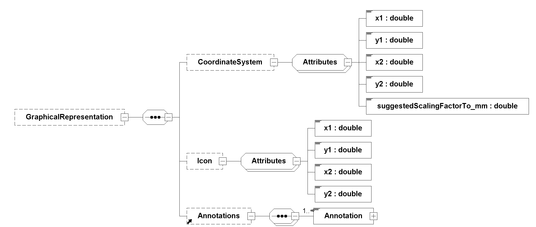
2.4.9.1.2. CoordinateSystem
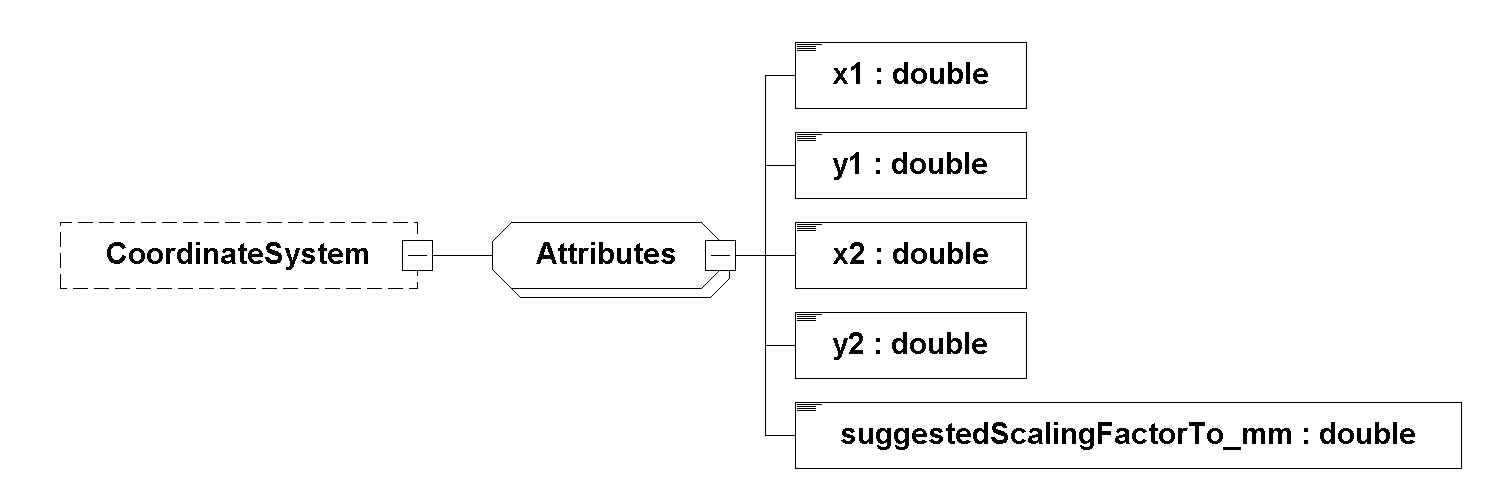
The <CoordinateSystem> element and its extent is used as reference for other graphical items.
It also provides a scaling factor to millimeter.
The coordinate system is defined by the coordinates of two points, the lower left (x1, y1) corner and the upper right (x2, y2) corner, where the coordinates of the first point shall be less than the coordinates of the second point [a first quadrant coordinate system].
The x-axis is directed to the right, the y-axis is directed upwards.
[The exporting tool should define how the coordinate system unit relates to mm display or printout size. However, an importer might choose to use the factor from the default coordinate system extent to the actual coordinate system extent to calculate a scaling factor, to match the default icon size in the importer.
The area defined by the coordinate system is suggested to be used as "clickable icon size" in importers.
A <Terminal> might be placed outside of this area, therefore the visible bounding box has to be determined by the importer.]
The coordinate system default is x1=-100, y1=-100, x2=100, y2=100.
This extent is used if the <CoordinateSystem> element is missing.
The default suggestedScalingFactorTo_mm is 0.1.
So the default coordinate system display size should be 20 mm width and 20 mm height.
The FMU icon and all graphical representations provide the position and extent with the attributes x1, y1, x2, y2.
The values of these attributes directly relate to this coordinate system and are not normalized.
Flipping of the FMU icon or a terminal can be realized by setting its attributes x2 < x1 or y2 < y1 without changing the coordinate system.
2.4.9.1.3. Icon
The extent and position of the FMU icon are defined in the <Icon> element.
The optional image file of the FMU icon is placed at the path terminalsAndIcons/icon.png in the ZIP archive of the FMU.
The terminals should not be visible in the image.
Optionally an SVG file with path terminalsAndIcons/icon.svg can be provided if also the PNG file is present.
This enables high quality rendering and printing in importers.
The point (x1, y1) maps to the left lower corner of the PNG image or SVG viewport.
The point (x2, y2) maps to the right upper corner of the PNG image or SVG viewport.
2.4.9.1.4. Placement, Extent, and Painting Order of Graphical Items

The clickable icon size is defined by the <CoordinateSystem> element.
The FMU icon itself may exceed this extent (or bounding box).
The bounding box of the terminals is given by the extent in the terminals element.
Their location is neither limited to the extent of the icon nor the extent of the coordinate system.
[An importer has to determine the outer bounding box enclosing all graphical items.]
Transparent SVG or PNG files are allowed and wanted.
The order of the elements in the XML file defines the order of painting.
The first element in the <TerminalGraphicalRepresentation> is painted first and therefore behind the others, the last element is painted on top of the others and because of that in front of them.
[So the FMU icon should be placed first in the XML file, terminal below.]
2.4.9.2. Definition of Terminals
2.4.9.2.1. Overview
Terminals are fully optional and can be ignored by any importer.
A terminal is:
-
a structured interface for connections to other models,
-
intended to be used for signal flow between models, parameter propagation, and compatibility checks of the model configuration, and
-
a sequence of references to variables with connection meta data.
Predefined rules for variable matching in a connection are given in Table 26. Predefined variable kinds are used to describe how the terminal member variables have to be handled. Domain specific connection rules, terminals and their member variables can be provided by other standards.
[Algebraic loops in systems of connected FMUs are not addressed or resolved by the terminals.
The FMU standard does not require that the causality of the terminal member variables in connected terminals match.
This must be handled by the importer.
The System Structure & Parameterization Standard (SSP) refers to a connectorKind.
This connectorKind is not related to the terminalKind or variableKind described in Section 2.4.9.2.2 and Section 2.4.9.2.3.]
2.4.9.2.2. Terminals
Element <fmiTerminalsAndIcons><Terminals> is defined as:
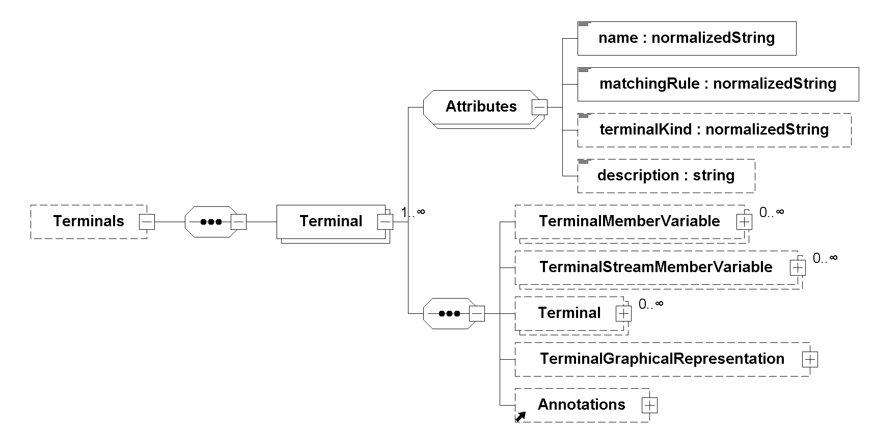
The normalized string attribute name of the <Terminal> element is the unique instance name of the terminal.
The terminal name must be unique on each level.
The normalized string attribute matchingRule describes the rules for variable matching in a connection of terminals.
As detailed in Table 26, there are three predefined matching rules: plug, bus, and sequence.
Other standards may define new matching rules.
In order to avoid ambiguities and conflicts, rule names must follow the reverse domain notation of a domain that is controlled by the entity defining the semantics and content of the additional entries.
The rule names beginning with org.modelica and org.fmi-standard are explicitly reserved for use by layered standards defined by Modelica Association or its own projects (MAPs).
The normalized string terminalKind is an optional attribute.
Other standards may define terminal kinds.
It is intended that the terminalKind is used to define domain specific member variable sequences, member names and order, or high level restrictions for connections.
[Externally defined terminal kinds should refer to a predefined matchingRule, if possible.
Vendor specific terminal kinds should start with _vendorName or _toolName to avoid namespace clashes.
Examples for terminalKind: StandardXXX_Mechanical_Translational, Modelica.Mechanics.Translational.Interfaces.Flange_a, vendorNameA_customTypeA, _vendorNameB_customLibrary_customTypeB.
The structured naming convention of the <ModelVariables> is independent from the terminal names and member variable names.
A tool may choose to connect terminals with a different or unknown terminalKind, if the matchingRule matches.]
2.4.9.2.3. Terminal Member Variable
The <TerminalMemberVariable> is defined as:
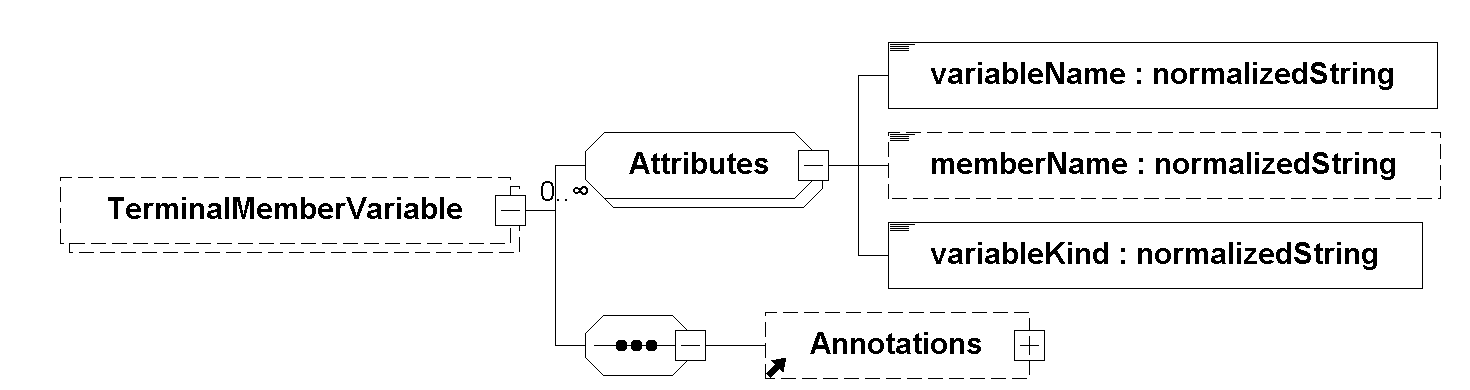
The normalized string variableName identifies a variable in <ModelVariables> which is actually connected and for which fmi3Get{VariableType} and fmi3Set{VariableType} is called.
If the matchingRule plug and bus are used, then memberName is used for variable matching.
Therefore, the memberName attribute is required for plug and bus and must be unique per terminal.
The memberName is not required for matchingRule sequence.
The normalized string variableKind is used to provide general information about the variable.
This information defines how the connection of this variable has to be implemented (e.g. Kirchhoff’s current law or common signal flow).
The predefined variableKind are:
.Predefined kinds of variables.
variableKind |
Description |
|---|---|
|
The values in connected terminals are intended to be equal.
Restricted to |
|
Variables which fulfill Kirchhoff’s current law.
Restricted to |
[The suggested variable naming scheme for the structured naming convention is <ModelVariable name> = <terminalName>.<memberName>.
Not all <ModelVariables> which have the prefix "<terminalName>." are a member variable, and there may exist member variables which don’t have this prefix.
Example 1 (suggested scheme): <ModelVariable name> is portA.U, <terminalName> is portA, <memberName> is U.
Example 2 (suggested scheme): <ModelVariable name> is hierarchConn.innerConn.U, <outer terminal name> is hierarchConn, <inner terminal name> is innerConn, <memberName> is U.
Example 3 (no prefix): <ModelVariable name> is u, <terminalName> is portA, <memberName> is u.
Example 4 (prefix but not a member): <ModelVariable name> is portA.u, there is a terminal with <terminalName> portA, but this variable is not a terminal member.
The suggested variable naming scheme for the non-structured naming convention is: <ModelVariable name> = <memberName>
Matching is not restricted by variability, causality or variable type.
Example: A fixed variable may be connected to a tunable variable, a variable of type fmi3Float64 may be connected to a variable of type fmi3Int32.
However, it is recommended that the variable types and variabilities are equal.
The matchingRule refers to the <TerminalMemberVariable> on the same level only.
Nested terminals can have different matchingRules.
There is no special handling of derivatives.
If a derivative is a terminal member variable then it is considered as normal member variable.
However, if a derivative of a terminal member variable is not terminal member, then this derivative information may be used by an importer.]
2.4.9.2.4. Terminal Stream Member Variable
The <TerminalStreamMemberVariable> is defined as:
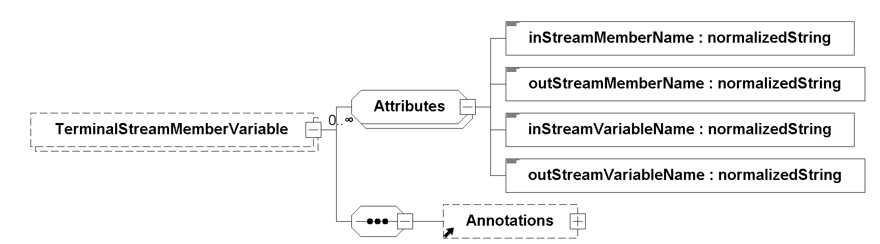
This element is used for variables which fulfill the balance equation for transported quantities.
It is restricted to input and output, parameter and calculatedParameter.
The Stream concept is described in the appendix D "Derivations of Stream Equations" of the Modelica Language Specification.
Only one terminal member variable with the variableKind inflow or outflow per terminal is allowed, if a <TerminalStreamMemberVariable> is present.
[More sophisticated structures can be implemented using hierarchical terminals.]
The attribute inStreamVariableName and outStreamVariableName are used to identify the <ModelVariables>.
If the referenced model variables are arrays, then the size of the inStreamVariableName and outStreamVariableName has to be equal.
A terminal may have more than one <TerminalStreamMemberVariable>.
The inStreamMemberName and outStreamMemberName describe the terminal member name for matching purposes, similar to the memberName attribute in the <TerminalMemberVariable>.
[An example of use for an array of stream variables is a gas mixture flow.
The gas composition could be implemented as a mass fraction vector.
The outStreamVariableName refers to \(portA.q_\textit{outStream}\textit{[]}\) and the inStreamVariableName refers to \(portA.q_\textit{inStream}\textit{[]}\) .
The inStreamMemberName and outStreamMemberName are " \(q_\textit{inStream}\textit{[]}\) " and " \(q_\textit{outStream}\textit{[]}\) ".
Balance equation for transported quantities:
\(0 = \sum{q_i\dot{m}_i}\)
\(0 = \sum{\dot{m}_i}\cdot \left\{\begin{array}{ll} q_{i, \mathit{outStream}} &\textit{if $\dot{m}$ is outflowing through terminal $i$}\\ q_{i, \mathit{inStream}} &\textit{if $\dot{m}$ is inflowing through terminal $i$} \end{array}\right.\)
The \(q_{i,\mathit{outStream}}\) is the convective quantity in case the matter flows out of the FMU.
\(q_{i,\mathit{inStream}}\) is the convective quantity in case the matter flows into the FMU.
Both variables are present in the terminal.
The outStream variable has the causality output or calculatedParameter because this information has to be provided by each FMU.
The inStream variable has the causality input or parameter.
To display the actual value in an importer, this actual value has to be selected depending on the sign of the terminal member variable with variableKind inflow or outflow.
However, calculating the actual value is not necessary.
If only two terminals with a variable are connected and their causality matches, then the values of the outStream variables can be forwarded to the corresponding inStream values.
In Modelica the inStream variable is not directly visible, the value can only be accessed using "inStream()", therefore an additional model variable has to be added during the export. It is suggested that Modelica tools exporting an FMU derive the member name for the inStream variable according to the scheme "<outStream name>_inStream". E.g. if the outStream name is "h_outflow" then the inStream name should be "h_outflow_inStream".]
2.4.9.2.5. Terminal Graphical Representation
The <TerminalGraphicalRepresentation> is defined as:
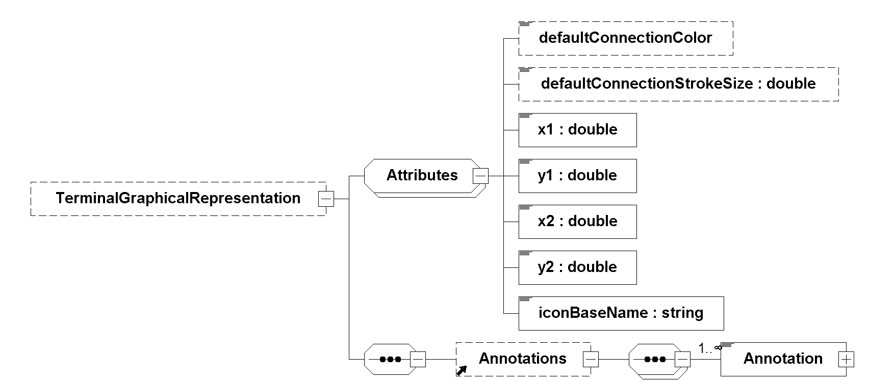
The iconBaseName attribute is mandatory.
This attribute defines the base name of the image file as a relative URI according to RFC 3986.
The base URI that this relative URI is resolved against is the URI of the terminalsAndIcons/terminalsAndIcons.xml file in the FMU ZIP archive.
Implementations are required to support relative URIs, excluding relative URIs that move beyond the baseURI (i.e. go "up" a level via ..).
Implementations are not required to support any absolute URIs and any specific URI schemes.
The PNG file with the extension '.png' has to be provided.
An additional SVG file with extension '.svg' is optional.
[Note that this specification is functionally equivalent to looking up image sources from the terminalsAndIcons folder of the FMU ZIP archive after dot removal from the path as per section 5.2.4 of RFC 3986.]
The defaultConnectionStrokeSize and defaultConnectionColor can be provided to define the intended connection line layout in the importer.
The stroke size is given relative to the coordinate system extent.
The stroke color is given in RGB values from 0 to 255. E.g.: 255 255 0.
[Nested terminals may have a <TerminalGraphicalRepresentation> element.
However, if and how nested terminals are displayed, is up to the importer.]
[The order of painting of the <TerminalGraphicalRepresentation> of terminals on each level is equal to the order in the <Terminal> element.
So graphical representations appearing first, are painted first, are behind graphical representations which appear below.]
The Annotations element can be used by vendors to store additional information for the graphical representation.
[It is suggested that Modelica tools store the Modelica annotation of the connector under the type org.modelica.Modelica4Annotation in the annotations of an element connector.
The attribute name of the connector element is equal to the name attribute of the referenced fmi3Terminal.]
2.4.9.2.6. General Remark on Signal
[The signal variableKind can be applied for different use cases.
The first use case is a signal flow from an output of one FMU to an input of another FMU.
The output value has to be forwarded to the input.
The signal flow can cause algebraic loops.
If variables in connected terminals have the causality output, then an importer may iterate an undefined input of an FMU to ensure that the connected output values are equal.
Another use case is the parameter propagation.
If a variable in both connected terminals has the causality parameter, then an importer could ask the user for the value of one of those parameters only, and propagate this value to the other FMU.
If only one of the variables has causality parameter, and the other is a constant output or calculatedParameter, then the importer could also propagate the parameter value without presenting a parameter to the user.
One example of use would be the name of a substance flowing through a pipe.
If the fluid flows from one pipe FMU to another, the substance should be the same.
This substance name could be propagated over several FMUs.
Finally the variableKind signal can be applied to implement compatibility checks.
If for example the variability of the variables in connected terminals are constant, then the importer can implement an equality assertion.
This is also possible with calculated parameters.
One example of use would be the cross sectional flow area in pipes which is calculated from geometry parameters.
A change in the cross sectional flow area is relevant for the momentum equation, and therefore the connection has to be deemed incompatible if these variables are present and unequal.]
2.4.9.2.7. General Remark on Inflow and Outflow
[Flow variables have a direction and must fulfill a zero sum constraint i.e. the sum of all flow variables connected must be zero (Kirchhoff’s current law).
In addition because different tools might have different direction definitions both, inflow and outflow are available as variableKind.
For variables with inflow a positive value means that the flow is inwards, and for outflow a positive value means that the flow is outwards.
For the sake of simplicity in the following \(\dot{m}_i\) denotes an inflowing quantity:
\(0 = \sum{\dot{m}_i}\)
[Connecting a single output outflow to a single input inflow, or vice versa automatically fulfills the flow constraint, while connecting two variables of the same flow type requires a negation of the variable value.
inflow and outflow is only used as a sign convention for scalar flow quantities which obey Kirchhoff’s current law (sum up to zero).
Other, nonscalar, quantities which also sum up to zero, like a mechanical force in 3D space according to D’Alembert’s principle, are not covered by this sign convention.
This is the case since Kirchhoff’s current law only holds for scalars where a sign convention is sufficient.
Other definitions are beyond the scope of this terminal specification and need clear definition in other specifications on top of this.]
2.4.10. Build Configurations
Each <BuildConfiguration> provides the necessary information to compile and link the sources of the model into a dynamic library or as part of an executable.
An FMU importer may not regard more than one <BuildConfiguration> when building the FMU for a specific platform.
The importer chooses the matching <BuildConfiguration> based on the platform and modelIdentifier attributes.
[On platforms that support shared libraries, executables should not be linked statically against or be compiled directly from the sources of an FMU in order to avoid name conflicts.]
In order to avoid symbol name conflicts when compiling and linking multiple source code FMUs, source files should keep the exported symbols to a minimum by declaring all symbols not needed for linking as static.
If only a single <SourceFile> is provided in the <BuildConfiguration> all symbols except for the FMI functions should be defined as static.
This source file may include other source files that are not listed in the <BuildConfiguration>.
It is also recommended to use a descriptive name (e.g. <model_identifier>.c) for this single <SourceFile> instead of generic names (like all.c, or model.c) in order to aid readability and reduce integration effort.
| Attribute | Description |
|---|---|
|
The attribute |
|
Platform tuple of the platform the |
|
Description of the build configuration |
2.4.10.1. SourceFileSet
The <SourceFileSet> element groups source files that can be compiled with the same compiler and compiler options.
Every build configuration must contain at least one <SourceFileSet>.
An importer of the FMU has to process every <SourceFileSet> of the matching <BuildConfiguration>.
| Attribute | Description |
|---|---|
|
Unique name of the |
|
Language of the source files (e.g. |
|
The compiler to compile the sources (e.g. |
|
The compiler flags that have to be used when compiling the sources (e.g. |
2.4.10.2. SourceFile
| Attribute | Description |
|---|---|
|
Path of the source file relative to the |
2.4.10.3. PreprocessorDefinition
The <PreprocessorDefinition> element defines a preprocessor definition that needs to be passed to the compiler when compiling the source files in the <SourceFileSet>.
| Attribute | Description |
|---|---|
|
Name of the preprocessor definition |
|
Value of the preprocessor definition |
|
Determines whether the definition is optional (default is |
|
Description of the preprocessor definition |
2.4.10.4. PreprocessorDefinition/Option
The <Option> element defines a possible value for the <PreprocessorDefinition>.
If a <PreprocessorDefinition> contains <Option> elements, its default value must be contained in the options.
| Attribute | Description |
|---|---|
|
Value of the preprocessor definition option |
|
Description of the preprocessor definition option |
2.4.10.5. IncludeDirectory
The <IncludeDirectory> element defines the include directories that need to be passed to the compiler when compiling the source files in the <SourceFileSet>.
| Attribute | Description |
|---|---|
|
Path of the include directory relative to the |
[Note that the header files fmi3PlatformTypes.h and fmi3FunctionTypes.h/fmi3Functions.h are not included in the FMU because:
fmi3PlatformTypes.h makes no sense in the sources directory, because if sources are provided, then the importer defines this header file and not the FMU.
This header file is not included in the binaries directory, because it is implicitly defined by the platform directory (for example, x86-windows for a 32-bit machine running Windows or x86_64-linux for a 64-bit machine running Linux).
fmi3FunctionTypes.h / fmi3Functions.h are not needed in the sources directory, because they are implicitly defined by attribute fmiVersion in file modelDescription.xml.
Furthermore, in order that the C compiler can check for consistent function arguments, the header file from the importer should be used when compiling the C sources.
It would therefore be counter-productive (unsafe) if this header file was present.
These header files are not included in the binaries directory, since they are already utilized to build the executable of the simulation environment.
The version number of the header file used to construct the FMU can be deduced via attribute fmiVersion in file modelDescription.xml or via function call fmi3GetVersion.]
2.4.10.6. Library
The <Library> element defines a static library required to link the model binary.
An importer of the FMU has to link every library of the matching <BuildConfiguration>.
| Attribute | Description |
|---|---|
|
Name of the library |
|
Version specifier of the library as defined in PEP 440.
The characters |
|
Boolean attribute that determines whether the library is contained in the |
|
Description of the library definition option |
2.4.10.7. Examples
<?xml version="1.0" encoding="UTF-8"?>
<fmiBuildDescription fmiVersion="3.0">

  <BuildConfiguration modelIdentifier="PIDContoller">
    <SourceFileSet>
      <SourceFile name="PIDContoller.c"/>
    </SourceFileSet>
  </BuildConfiguration>

</fmiBuildDescription><?xml version="1.0" encoding="UTF-8"?>
<fmiBuildDescription fmiVersion="3.0">
<BuildConfiguration modelIdentifier="PlantModel" description="Build configuration for desktop platforms">
<SourceFileSet language="C99">
<SourceFile name="fmi3Functions.c"/>
<SourceFile name="solver.c"/>
</SourceFileSet>
<SourceFileSet language="C++11">
<SourceFile name="model.c"/>
<SourceFile name="logging/src/logger.c"/>
<PreprocessorDefinition name="FMI_VERSION" value="3"/>
<PreprocessorDefinition name="LOG_TO_FILE" optional="true"/>
<PreprocessorDefinition name="LOG_LEVEL" value="0" optional="true">
<Option value="0" description="Log infos, warnings and errors"/>
<Option value="1" description="Log warnings and errors"/>
<Option value="2" description="Log only errors"/>
</PreprocessorDefinition>
<IncludeDirectory name="logging/include"/>
</SourceFileSet>
<Library name="hdf5" version=">=1.8,!=1.8.17,<1.10" external="true" description="HDF5"/>
</BuildConfiguration>
<BuildConfiguration modelIdentifier="PlantModel" platform="aarch64-linux">
<SourceFileSet language="C99">
<SourceFile name="fmi3Functions.c"/>
</SourceFileSet>
<SourceFileSet language="C++11" compiler="clang++" compilerOptions="-fno-rtti">
<SourceFile name="model.c"/>
<PreprocessorDefinition name="NO_FILE_SYSTEM"/>
</SourceFileSet>
<Library name="libm.a" description="OpenLibm math library"/>
</BuildConfiguration>
</fmiBuildDescription>2.5. FMU Distribution
An FMU consists of several files, that are stored in a ZIP file with a pre-defined structure.
The implementation of the FMI C-API may be distributed in source code and/or in binary format.
The FMU must be distributed with at least one implementation, in other words, either sources or one of the binaries for a particular machine.
It is also possible to provide the sources and binaries for different target machines together in one ZIP file.
The FMU must implement all common API functions according to Section 2.2 and the functions for at least one of the interface types.
Especially it is required that all functions that are part of the specified interface type are present, even if they are only needed for optional capabilities that the FMU does not support.
The behavior of those functions is unspecified, so while calling environments can rely on the functions being present, they cannot rely on any particular behavior for functions only needed for capabilities the FMU does not support.
Additional functions may be present in the FMU, as for example required by the OS ABI, for layered standards, or future FMI versions.
All symbols starting with the prefix fmi3 are reserved for use in future minor releases of FMI 3.0.
The extension of the ZIP file must be .fmu [, for example, HybridVehicle.fmu].
The compression method for all files stored in the ZIP archive must be either 8 (deflate), or 0 (store).
Only files stored using compression method 8 (deflate) may be stored with general purpose bit 3 set.
The field version needed to extract of the archive must not be higher than 2.0, and encryption must not be employed.
The archive must not be a split or spanned ZIP archive.
Links must not be used inside the ZIP archive.
[These restrictions ensure broad compatibility of the archive with common ZIP processing tools and libraries.)]
[Note: especially section 4.4.17 of the ZIP format specification states that backslashes "\" are forbidden as path separator, only forward slashes "/" are allowed.
Non-ASCII directory names are not explicitly forbidden, but might pose a problem on different operating systems and are thus discouraged.]
Every FMU is distributed with its own ZIP file.
2.5.1. Structure of the ZIP file
modelDescription.xml                // description of FMU (required file)
documentation                       // directory containing the documentation (optional)
   index.html                       // entry point of the documentation
   diagram.png                      // descriptive diagram view of the model (optional)
   diagram.svg                      // if provided, diagram.png is also required (optional)
   externalDependencies.{txt|html}  // documentation of external resources required to load
                                    // or simulate the FMU
   <other documentation files>
   licenses                         // directory for licenses (optional)
      license.{txt|html|spdx}       // entry point for license information
      <license files>               // for example BSD licenses (optional)
   staticLinking.{txt|html}         // entry point for static link information (optional)
terminalsAndIcons                   // FMU and terminal icons (optional)
   terminalsAndIcons.xml            // description of terminals and icons (optional)
   icon.png                         // image file of icon without terminals (optional)
   icon.svg                         // if existing the icon.png is required (optional)
                                    // all terminal and fmu icons referenced in the
                                    // graphical representation
sources                             // directory containing the C sources (optional)
   buildDescription.xml
binaries                            // directory containing the binaries (optional)
   x86_64-windows                   // binaries for Windows on Intel 64-bit
      <modelIdentifier>.dll         // shared library of the FMI implementation
      <other DLLs>                  // the DLL can include other DLLs
   x86-linux                        // binaries for Linux on Intel 32-bit
      <modelIdentifier>.so          // shared library of the FMI implementation
   aarch32-linux                    // binaries for Linux on ARM 32-bit
      <modelIdentifier>.so          // shared library of the FMI implementation
   x86_64-darwin                    // binaries for macOS
      <modelIdentifier>.dylib       // shared library of the FMI implementation
resources                           // resources used by the FMU (optional)
extra                               // Additional (meta-)data of the FMU (optional)
2.5.1.1. Directory documentation
Figure Structure of the ZIP file of an FMU defines the files expected in the documentation directory.
If the FMU depends on external resources [e.g. shared libraries, files, or servers] to be loaded or simulated documentation/externalDependencies.{txt|html} must be present to document these dependencies and how to provide them.
2.5.1.1.1. Directory licenses
This optional subdirectory can be used to bundle all license texts for the code, binaries or other material (documentation, content of resources folder) contained in the FMU.
If it is present, it must contain either a license.spdx, license.txt or license.html file as entry point.
[It is strongly recommended to include all license and copyright related information in the licenses folder of an FMU (especially but not only for contained open source software) - the license.{txt|html} file can serve as an entry point for describing the contained licenses.
This will help the users to comply with license conditions when passing source or binary code contained in an FMU to other persons or organizations.]
2.5.1.2. Directory terminalsAndIcons
See Section 2.4.9 for a definition of the directory terminalsAndIcons.
2.5.1.3. Directory sources
A source code FMU contains the sources of the model in the sources directory together with a buildDescription.xml that contains at least one <BuildConfiguration> element for the supported platforms.
The header files fmi3PlatformTypes.h, fmi3FunctionTypes.h and fmi3Functions.h are not included in the FMU, but supplied by the importer to potentially reflect their specific platform and compiler tool set.
2.5.1.4. Directory binaries
A binary FMU must contain the binary files for all supported platforms in this folder.
To use the binaries of a specific platform, all items in that platform-specific binary folder must be unpacked at the same location as the binary <modelIdentifier>.{dll|dylib|so}.
2.5.1.4.1. Platform Tuple Definition
The names of the binary directories are standardized by the "platform tuple".
Further names can be introduced by vendors.
FMUs should contain all resources that are required to load and execute a shared library, link against a static library, or compile from source.
Shared libraries should be statically linked against their dependencies [e.g. the Visual Studio C Runtime on Windows].
RPATH="$ORIGIN" should be set when building ELF binaries to allow dynamic loading of dependencies on the target machine.
All external dependencies must be documented (see Section 2.5.1.1).
The binaries must be placed in the respective <platformTuple> directory with the general format <arch>-<sys>.
- Architecture
<arch> -
Name Description aarch32
ARM 32-bit Architecture
aarch64
ARM 64-bit Architecture
x86
Intel/AMD x86 32-bit
x86_64
Intel/AMD x86 64-bit
- Operating system
<sys> -
Name Description darwin
Darwin (macOS, iOS, watchOS, tvOS, audioOS)
linux
Linux
windows
Microsoft Windows
When shipping the implementation as a static library an optional ABI (Application Binary Interface) directory <arch>-<sys>{-<abi>} may be added to separate binaries for different toolchains on the same platform and a description must be provided in documentation/staticLinking.{txt|html} that contains all necessary information to link against the provided library [e.g. supported compilers].
The ABI directory must only contain lowercase characters a…z, digits 0…9, and underscores and start with a lowercase character a…z _[e.g. x86_64-windows-msvc140mt for a static library for 64-bit Windows generated with Visual Studio 2015 with /MT flag].
2.5.1.4.2. Platform Tuple Examples
The following table lists the most common platform tuples for shared libraries and the corresponding FMI 2.0 platform.
| Name | FMI 2.0 | Description |
|---|---|---|
x86_64-darwin |
darwin64 |
macOS on 64-bit x86 |
aarch64-darwin |
macOS on Apple Silicon |
|
x86-linux |
linux32 |
Linux on 32-bit x86 |
x86_64-linux |
linux64 |
Linux on 64-bit x86 |
aarch64-linux |
Linux on ARM64 |
|
x86-windows |
win32 |
Windows on 32-bit x86 |
x86_64-windows |
win64 |
Windows on 64-bit x86 |
aarch64-windows |
Windows on ARM64 |
2.5.1.4.3. External Libraries
If runtime libraries are needed by the FMU that have to be present on the target machine and cannot be shipped within the FMU (e.g., due to licensing issues), then automatic processing is likely impossible.
In such cases special handling is needed, for example, by providing the runtime libraries at appropriate places by the receiver.
The requirements and the expected processing must be documented in the documentation directory in the file externalDependencies.{txt|html}.
2.5.1.5. Directory resources
In the optional directory resources, additional data can be provided in FMU specific formats, typically for tables and maps used in the FMU.
More folders can be added under resources (tool/model specific).
For the FMU to access these resource files, the resources directory shall be available in extracted form and the absolute path to this directory is provided via argument resourcePath of fmi3InstantiateXXX.
The resources directory must be available for the lifetime of the FMU instance.
The FMU instance must not write to or delete the directory or parts of it.
2.5.1.6. Directory extra
The ZIP archive may contain additional subdirectories within extra/ that can be used to store additional data, e.g. for the implementation of layered standards.
In order to avoid ambiguities and conflicts, the names of these subdirectories should use the reverse domain notation of a domain that is controlled by the entity defining the semantics and content of the additional entries [(for example extra/com.example/SimTool/meta.xml or extra/org.example.stdname/data.asd)].
The use of subdirectories beginning with org.modelica and org.fmi-standard is explicitly reserved for use by layered standards defined by Modelica Association or its own projects (MAPs), i.e. layered standards defined outside the Modelica Association must not use subdirectory names beginning with these prefixes.
It is explicitly allowed for tools and users other than the original creator of an FMU to modify, add or delete entries in the extra/ directory without affecting the validity of the FMU in all other aspects.
Specifically all validation or digital signature schemes used to protect the content of the FMU should take the variability of extra file content into account [(for example by having separate checksums or signatures for FMU core content and extra content, or not having signatures at all for extra content)].
2.5.2. Multiple Interface Types
One FMU may implement multiple FMI types.
Such an FMU may be used by differently capable simulation algorithms and for different use cases.
To indicate support for a specific interface type, the <fmiModelDescription> must have the respective element present.
Supported interface types may be provided differently, as binary and/or source code.
[Example of different libraries:
   binaries
     x86_64-windows
        MyModel_ModelExchange.dll      // modelIdentifier of <ModelExchange> =
                                       //    "MyModel_ModelExchange"
        MyModel_CoSimulation.dll       // modelIdentifier of <CoSimulation> =
                                       //    "MyModel_CoSimulation"
]
Support of multiple interface types in one FMU is possible only, if the interface variables are identical.
2.5.3. Dependency on Installed Tool
If an FMU depends on services provided by an external tool, then needsExecutionTool = true.
These tool dependencies must be documented.
2.5.4. Import Examples
The following code examples demonstrate how to access the FMI functions of FMUs that are implemented as a shared library or static library / source code.
2.5.4.1. Accessing FMI Functions in Shared Libraries
/* This example demonstrates how to import an FMU implemented as a shared library */

#ifdef _WIN32
#include <Windows.h>
#else
#include <dlfcn.h>
#endif

#include <stdlib.h>

// FMI function types
#include "fmi3FunctionTypes.h"

#define INSTANTIATION_TOKEN "{8c4e810f-3da3-4a00-8276-176fa3c9f000}"


static void cb_logMessage(fmi3InstanceEnvironment instanceEnvironment, fmi3Status status, fmi3String category, fmi3String message) {
    // log message...
}

int main(int argc, char* argv[]) {

#if defined(_WIN32)
    HMODULE libraryHandle = LoadLibraryA("VanDerPol\\binaries\\x86_64-windows\\VanDerPol.dll");
#elif defined(__APPLE__)
    void *libraryHandle = dlopen("VanDerPol/binaries/x86_64-darwin/VanDerPol.dylib", RTLD_LAZY);
#else
    void *libraryHandle = dlopen("VanDerPol/binaries/x86_64-linux/VanDerPol.so", RTLD_LAZY);
#endif

    if (!libraryHandle) {
        return EXIT_FAILURE;
    }

    fmi3InstantiateModelExchangeTYPE *instantiateModelExchange = (fmi3InstantiateModelExchangeTYPE *)
#ifdef _WIN32
        GetProcAddress(libraryHandle, "fmi3InstantiateModelExchange");
#else
        dlsym(libraryHandle, "fmi3InstantiateModelExchange");
#endif

    fmi3FreeInstanceTYPE *freeInstance = (fmi3FreeInstanceTYPE *)
#ifdef _WIN32
        GetProcAddress(libraryHandle, "fmi3FreeInstance");
#else
        dlsym(libraryHandle, "fmi3FreeInstance");
#endif

    // load remaining FMI functions...

    if (!instantiateModelExchange || !freeInstance) {
        return EXIT_FAILURE;
    }

    fmi3Instance m = instantiateModelExchange(
        "instance1",         // instance name
        INSTANTIATION_TOKEN, // instantiation token (from XML)
        NULL,                // resource path
        fmi3False,           // visible
        fmi3False,           // debug logging disabled
        NULL,                // instance environment
        cb_logMessage);      // logger callback


    if (!m) {
        return EXIT_FAILURE;
    }

    // simulation...

    freeInstance(m);

    // unload shared library
#ifdef _WIN32
    FreeLibrary(libraryHandle);
#else
    dlclose(libraryHandle);
#endif

    return EXIT_SUCCESS;
}
2.5.4.2. Accessing FMI Functions in Static Libraries and Source Code
/* This example demonstrates how to import an FMU implemented as a static library or source code*/

// FMI function prefix (from XML)
#define FMI3_FUNCTION_PREFIX VanDerPol_
#include "fmi3Functions.h"
#undef FMI3_FUNCTION_PREFIX

#define INSTANTIATION_TOKEN "{8c4e810f-3da3-4a00-8276-176fa3c9f000}"


static void cb_logMessage(fmi3InstanceEnvironment instanceEnvironment, fmi3Status status, fmi3String category, fmi3String message) {
    // log message
}

int main(int argc, char* argv[]) {

    fmi3Instance m = VanDerPol_fmi3InstantiateModelExchange(
        "instance1",         // instance name
        INSTANTIATION_TOKEN, // instantiation token (from XML)
        NULL,                // resource location
        fmi3False,           // visible
        fmi3False,           // debug logging disabled
        NULL,                // instance environment
        cb_logMessage);      // logger callback

    // simulation ...

    VanDerPol_fmi3FreeInstance(m);

    return m ? EXIT_SUCCESS : EXIT_FAILURE;
}
2.6. Versioning and Layered Standards
The FMI standard uses semantic version numbers, as defined in [PW13], where the standard version consists of a triple of version numbers, consisting of major version, minor version, and patch version numbers [e.g. 1.2.3 for major version 1, minor version 2 and patch version 3].
-
Major versions will introduce changes that are neither backward nor forward compatible, including changes to the XML schemas to include new non-ignorable content.
-
Minor versions will only contain clarifications and include new layered standards, which may add new ignorable XML content, as defined below, into the core standard document, indicating that the standard needs to be supported by all conforming implementations.
-
Patch versions will only change explanatory text of the standard, make formerly defined content clearer, without any other changes to the XML schemas or other content definitions. For this reason, the version number attribute of all FMI files will only contain major and minor version numbers and not the patch version number: It should never be necessary for an importer to know the patch version number of the standard that the generating tool implemented.
In order to enable the backward-compatible extension of the FMI standard in minor releases and between minor releases, the FMI project intends the use of the layered standard mechanism to introduce new features in a fully backward-compatible and optional way.
A layered standard defines extensions to the base FMI standard by specifying, for example:
-
support for additional MIME types,
-
new values for
matchingRuleorterminalKindfor Terminals and/or -
adding C-API functions/variables.
Any FMU following a layered standard on top of FMI 3.0 must still be a compliant FMI 3.0 FMU.
Layered standards can fall into one of three categories:
Layered standards that have achieved enough adoption or importance to be included into the base standard could be incorporated into a new minor or major release version of the base standard, making support for this layered standard optional or required for conformance with the newly published release of the FMI standard.
3. FMI for Model Exchange
FMI for Model Exchange provides a standardized interface for solving ordinary differential equations with events (abbreviated as "hybrid ODE"). In contrast to FMI for Co-Simulation, a Model Exchange FMU implements the model algorithm only, without the required solution method.
The importer controls the data exchange and the synchronization between FMUs.
The solver algorithm itself is not part of the FMI standard.
The solver algorithm is responsible for:
-
advancing the overall simulation time,
-
exchange input and output data,
-
computation of continuous state variables by time integration,
-
triggering of input clocks, and
-
handling events.
In contrast to Co-Simulation, the FMU is evaluated only at a specific time instant and not from one communication point to the next. A Model Exchange FMU might consist of discrete-time equations only, for example, describing a sampled-data controller.
FMI for Model Exchange enables the following features:
-
explicit or implicit integration algorithms with constant or variable step size,
-
dedicated Initialization Mode, which allows computation of consistent initial conditions over algebraic loops,
-
exact localization of state events using event indicators,
-
solution of algebraic loops involving input and output variables of this FMU (see algebraic loops),
-
selective computation of FMU variables required by the solver algorithm, e.g. outputs, event indicators, derivatives (see Section 2.2.10),
-
the ability of the FMU to provide directional and adjoint partial derivatives.
Which of the features above are supported by a specific FMU is defined by capability flags.
3.1. Concepts
3.1.1. Localization of State Events
Integration algorithms for differential equations assume continuous behavior of variables. In hybrid ODEs, there are points during the simulation, when this assumption is violated. A hybrid ODE solver must therefore:
-
locate exactly when such a discontinuity (event) happens and enter Event Mode. This is trivial for time events. For state events event indicators are used.
-
handle such events in Event Mode.
-
restart the integration algorithm when leaving Event Mode.
An event indicator, and only an event indicator, signals a state event with the domain change from \(\mathbf{z}_j > 0\) to \(\mathbf{z}_j \leq 0\) or from \(\mathbf{z}_j \leq 0\) to \(\mathbf{z}_j > 0\).
[This definition is slightly different from the usual standard definition of state events: \(\mathbf{z}(t) \cdot \mathbf{z}(t_{i-1}) \leq 0\) which has the severe drawback that the value of the event indicator at the previous event instant, \(\mathbf{z}(t_{i-1}) \neq 0\), must be non-zero and this condition cannot be guaranteed.
The often used term "zero-crossing function" for \(\mathbf{z}\) is misleading (and is therefore not used in this document), since a state event is defined by a domain change and not by a zero-crossing of a variable.]
The FMU must guarantee that after leaving Event Mode \(\mathbf{z}_j \neq 0\), for example, by shifting \(\mathbf{z}_j\) with a small value.
[All event indicators should be continuous between events.
Furthermore, \(\mathbf{z}_j\) should be scaled in the FMU with its nominal value (so all elements of the returned vector eventIndicators should be in the order of 1).]

During event localization the FMU might be evaluated after the switch of an event indicator. Even when an event indicator switches, its corresponding relation must stay "frozen" to assure the continuity assumption of the integration algorithm. This allows an integration algorithm to properly finish the current integration step.
In Table 4, vector \(\mathbf{r}\) is used to label all relations. In Continuous-Time Mode all these relations are "frozen". This is indicated in the mathematical description of Event Mode by computing \({}^\bullet\mathbf{r}\) when leaving Event Mode and using \({}^\bullet\mathbf{r}\) in the right-hand side of \({\mathbf{f}_{\mathit{cont}}}\) and \({\mathbf{f}_{\mathit{comp}}}\) in mathematical description of Continuous-Time Mode.
[Example: An assignment of the form
y = ((x1 > x2) || (x1 < x3)) ? +1 : -1;
can be implemented in the FMU as:
// event indicator computation:
z1 = x1 - x2;
z2 = x3 - x1;

// relations do not change in Continuous Time Mode
if Initialization Mode || Event Mode {
  r1 = z1 > 0;
  r2 = z2 > 0;
}
y = (r1 || r2) ? +1 : -1;
Therefore, the original if-clause is evaluated in this form only during Initialization Mode and Event Mode. A hysteresis should be added, in the FMU, for the event indicators to stabilize the event localization.]
3.2. State Machine for Model Exchange
The state machine in Figure 40 defines the allowed calling sequences for FMI for Model Exchange.

Common states are defined in Section 2.3, such as super states FMU State Settable and Initialized, states Instantiated, Configuration Mode, Reconfiguration Mode, Initialization Mode, Event Mode and Terminated.
3.2.1. State: Continuous-Time Mode
The Continuous-Time Mode is used to compute the values of all continuous-time variables between events by numerically solving ordinary differential and algebraic equations. All discrete-time variables are fixed during this phase and the corresponding discrete-time equations are not evaluated.
In this state, the continuous-time equations are active and integrator steps are performed by the importer.
| Equations and Actions | Functions Influencing Equations |
|---|---|
\(t := (\) |
|
Set continuous-time |
|
Set continuous-time states \(\mathbf{x}_{c}(t)\) |
|
\((\mathbf{y}_{c}, \mathbf{\dot{x}}_c, \mathbf{z}, \mathbf{w}_{c}) := \mathbf{f}_{\mathit{cont}}(\mathbf{x}_{c}, {}^\bullet\mathbf{x}_{d}, \mathbf{u}_{c}, {}^\bullet\mathbf{u}_{d}, \mathbf{p}, {}^\bullet\mathbf{r}, {}^\bullet\mathbf{b}, t)\) |
|
|
|
|
- Allowed Function Calls
- Function
fmi3SetTime -
typedef fmi3Status fmi3SetTimeTYPE(fmi3Instance instance, fmi3Float64 time);Set a new value for the independent variable (typically a time instant).
-
Argument
timeis the new value for the real part \(t_{R}\) of \(t := (t_{R}, 0)\). It refers to the unit of theindependentvariable.timemust be larger or equal to:-
the time at the second last call to
fmi3CompletedIntegratorStep, -
the time at the last call to
fmi3EnterEventMode.
[This allows limited simulation backward in time. As soon as an event occurs (
fmi3EnterEventModewas called), going back in time is impossible, becausefmi3EnterEventMode/fmi3UpdateDiscreteStatescan only compute the next discrete state, not the previous one.] -
- Function
fmi3Set{VariableType} -
Only for variables with
causality=inputandvariability=continuous. - Functions
fmi3Get{VariableType} -
Getting variables might trigger computations.
- Function
fmi3SetContinuousStates -
typedef fmi3Status fmi3SetContinuousStatesTYPE(fmi3Instance instance,
                                               const fmi3Float64 continuousStates[],
                                               size_t nContinuousStates);
Set new continuous state values.
-
Argument
continuousStatescontains the new values for each continuous state. The order of thecontinuousStatesvector must be the same as the ordered list of elements<ContinuousStateDerivative>in<ModelStructure>. Array variables are serialized as defined in Section 2.2.7.1. This order is also used in the arguments of the following functions:fmi3GetNominalsOfContinuousStates,fmi3GetContinuousStates, andfmi3GetContinuousStateDerivatives. -
Argument
nContinuousStatesis the size of thecontinuousStatesvector.[
fmi3Status = fmi3Discardshould be returned if the FMU rejects any of the state values because they, for example, violate min/max value restrictions.]
-
- Functions
fmi3Get{VariableType} -
Getting variables might trigger computations.
- Function
fmi3GetContinuousStates -
Returns the current continuous state vector.
- Function
fmi3GetContinuousStateDerivatives -
typedef fmi3Status fmi3GetContinuousStateDerivativesTYPE(fmi3Instance instance,
                                                         fmi3Float64 derivatives[],
                                                         size_t nContinuousStates);
Returns the first-order derivatives with respect to the independent variable (usually time) of the continuous states.
-
Return argument
derivativescontains the derivatives for each continuous state with the same convention for the order as defined forfmi3SetContinuousStates. -
Argument
nContinuousStatesis the size of thederivativesvector.[
fmi3Status = fmi3Discardshould be returned if the FMU was not able to compute the derivatives according to \(\mathbf{f}_{\mathit{cont}}\) because, for example, a numerical issue, such as division by zero, occurred.]
-
- Function
fmi3GetEventIndicators -
typedef fmi3Status fmi3GetEventIndicatorsTYPE(fmi3Instance instance,
                                              fmi3Float64 eventIndicators[],
                                              size_t nEventIndicators);
Returns the event indicators signaling state events by their sign changes.
-
Return argument
eventIndicatorscontains the values for the event indicators in the order defined by the ordered list of XML elements<EventIndicator>. -
Argument
nEventIndicatorsis the current size of theeventIndicatorsvector (seefmi3GetNumberOfEventIndicators).
[
fmi3Status = fmi3Discardshould be returned if the FMU was not able to compute the event indicators according to \(\mathbf{f}_{\mathit{cont}}\) because, for example, a numerical issue, such as division by zero, occurred.] -
- Function
fmi3CompletedIntegratorStep -
typedef fmi3Status fmi3CompletedIntegratorStepTYPE(fmi3Instance instance,
                                                   fmi3Boolean  noSetFMUStatePriorToCurrentPoint,
                                                   fmi3Boolean* enterEventMode,
                                                   fmi3Boolean* terminateSimulation);
This function is called after every completed step of the integrator provided the capability flag
needsCompletedIntegratorStep = true. The importer must have set valid values fortime,continuousinputsandcontinuousstates prior to calling this function to evaluate \(\mathbf{f}_{\mathit{comp}}\) with valid right-hand side data.-
Argument
noSetFMUStatePriorToCurrentPoint = fmi3Trueiffmi3SetFMUStatewill no longer be called for time instants prior to current time in this simulation run. -
The return argument
enterEventModesignals that the importer must callfmi3EnterEventModeto handle a step event. -
When
terminateSimulation = fmi3True, the FMU requests to stop the simulation and the importer must callfmi3Terminate.
When the importer has reached valid values for the current integration step and one or more event indicators change sign (with respect to the previously completed integrator step), then the importer has to determine the time instant of the sign change that is closest to the previously completed integrator step. This is usually performed by an iteration where time is varied and state variables are determined by interpolation. Function
fmi3CompletedIntegratorStepmust be called after this state event location procedure. The intended purpose of the function call is to indicate to the FMU that at this stage allinputsand state variables have valid (accepted) values. Afterfmi3CompletedIntegratorStepis called, it is still allowed to go back in time (callingfmi3SetTime) and inquire values of variables at previous time instants withfmi3Get{VariableType}[for example, to determine values of non-state variables at output points]. However, it is not allowed to go back in time over the previousfmi3CompletedIntegratorStepor the lastfmi3EnterEventModecall.[In this function the FMU might, for example:
-
Update delay buffers
-
Detect step events and request handling of step events:
-
for dynamic state selection: The FMU checks whether the dynamically selected states are still numerically appropriate. If not, the function returns with
enterEventMode = fmi3True, the importer will callfmi3EnterEventModeand in Event Mode the new mapping is computed by the FMU. -
for projection: FMUs that represent a DAE can project their continuous-time states onto the constraint manifold in
fmi3UpdateDiscreteStates.
The new mapping or projection values might require a reinitialization of continuous-time states, which must be signaled to the importer by returning from
fmi3UpdateDiscreteStateswithvaluesOfContinuousStatesChanged = fmi3True. -
The function
fmi3CompletedIntegratorStepis not used to detect time events or state events, for example, by comparing event indicators of the previous with the current call offmi3CompletedIntegratorStep. Time events and state events must be detected by the importer, which has to callfmi3EnterEventModein these cases, even if the returning fromfmi3CompletedIntegratorStepwithenterEventMode = fmi3False.] -
- Function
fmi3EnterEventMode -
typedef fmi3Status fmi3EnterEventModeTYPE(fmi3Instance instance);This function changes the state to Event Mode.
The importer must call
fmi3EnterEventModewhen any of the following conditions are met:-
time has reached
nextEventTimeas returned byfmi3UpdateDiscreteStates, or -
the signs of the event indicators signal an event according to Section 3.1.1, or
-
the FMU returned with
enterEventMode = fmi3Truefromfmi3CompletedIntegratorStep, or -
the importer plans discrete changes to inputs, or
-
an input Clock needs to be set.
-
- Function
fmi3GetDirectionalDerivative - Function
fmi3GetAdjointDerivative
3.3. Code Example
In the following example, the usage of the fmi3XXX functions is sketched in order to clarify the typical calling sequence of the functions in a simulation environment.
Furthermore, it is assumed that one FMU is directly integrated in a simulation environment.
If the FMU would be used inside another model, additional code is needed, especially initialization and event iteration have to be adapted.
    CALL(FMI3InstantiateModelExchange(S,
        INSTANTIATION_TOKEN, // instantiationToken
        resourcePath(),      // resourcePath
        fmi3False,           // visible
        fmi3False            // loggingOn
    ));

    // set the start time
    fmi3Float64 time = 0;

    // set start values
    CALL(applyStartValues(S));

    // initialize
    // determine continuous and discrete states
    CALL(FMI3EnterInitializationMode(S, fmi3False, 0.0, time, fmi3True, stopTime));

    CALL(applyContinuousInputs(S, false));
    CALL(applyDiscreteInputs(S));

    CALL(FMI3ExitInitializationMode(S));

    // intial event iteration
    while (discreteStatesNeedUpdate) {

        CALL(FMI3UpdateDiscreteStates(S,
            &discreteStatesNeedUpdate,
            &terminateSimulation,
            &nominalsOfContinuousStatesChanged,
            &valuesOfContinuousStatesChanged,
            &nextEventTimeDefined,
            &nextEventTime));

        if (terminateSimulation) {
            goto TERMINATE;
        }
    }

    CALL(FMI3EnterContinuousTimeMode(S));

#if NZ > 0
    // initialize previous event indicators
    CALL(FMI3GetEventIndicators(S, previous_z, NZ));
#endif

#if NX > 0
    // retrieve initial state x and
    // nominal values of x (if absolute tolerance is needed)
    CALL(FMI3GetContinuousStates(S, x, NX));
    CALL(FMI3GetNominalsOfContinuousStates(S, x_nominal, NX));
#endif

    // retrieve solution at t=Tstart, for example, for outputs
    // S->fmi3SetFloat*/Int*/UInt*/Boolean/String/Binary(m, ...)

    CALL(recordVariables(S, outputFile));

    int steps = 0;

    while (!terminateSimulation) {

        // detect input and time events
        inputEvent = time >= nextInputEventTime(time);
        timeEvent = nextEventTimeDefined && time >= nextEventTime;

        const bool eventOccurred = inputEvent || timeEvent || stateEvent || stepEvent;

        // handle events
        if (eventOccurred) {

            CALL(FMI3EnterEventMode(S));

            if (inputEvent) {
                CALL(applyContinuousInputs(S, true));
                CALL(applyDiscreteInputs(S));
            }

            nominalsOfContinuousStatesChanged = fmi3False;
            valuesOfContinuousStatesChanged   = fmi3False;

            // event iteration
            do {
                // set inputs at super dense time point
                // S->fmi3SetFloat*/Int*/UInt*/Boolean/String/Binary(m, ...)

                fmi3Boolean nominalsChanged = fmi3False;
                fmi3Boolean statesChanged   = fmi3False;

                // update discrete states
                CALL(FMI3UpdateDiscreteStates(S, &discreteStatesNeedUpdate, &terminateSimulation, &nominalsChanged, &statesChanged, &nextEventTimeDefined, &nextEventTime));

                // get output at super dense time point
                // S->fmi3GetFloat*/Int*/UInt*/Boolean/String/Binary(m, ...)

                nominalsOfContinuousStatesChanged |= nominalsChanged;
                valuesOfContinuousStatesChanged   |= statesChanged;

                if (terminateSimulation) {
                    goto TERMINATE;
                }

            } while (discreteStatesNeedUpdate);

            // enter Continuous-Time Mode
            CALL(FMI3EnterContinuousTimeMode(S));

            // retrieve solution at simulation (re)start
            CALL(recordVariables(S, outputFile));

#if NX > 0
            if (valuesOfContinuousStatesChanged) {
                // the model signals a value change of states, retrieve them
                CALL(FMI3GetContinuousStates(S, x, NX));
            }

            if (nominalsOfContinuousStatesChanged) {
                // the meaning of states has changed; retrieve new nominal values
                CALL(FMI3GetNominalsOfContinuousStates(S, x_nominal, NX));
            }
#endif
        }

        if (time >= stopTime) {
            goto TERMINATE;
        }

#if NX > 0
        // compute continous state derivatives
        CALL(FMI3GetContinuousStateDerivatives(S, der_x, NX));
#endif
        // advance time
        time = ++steps * fixedStep;

        CALL(FMI3SetTime(S, time));

        // apply continuous inputs
        CALL(applyContinuousInputs(S, false));

#if NX > 0
        // set states at t = time and perform one step
        for (size_t i = 0; i < NX; i++) {
            x[i] += fixedStep * der_x[i]; // forward Euler method
        }

        CALL(FMI3SetContinuousStates(S, x, NX));
#endif

#if NZ > 0
        stateEvent = fmi3False;

        if (eventOccurred) {
            // reset the previous event indicators
            CALL(FMI3GetEventIndicators(S, previous_z, NZ));
        } else {
            // get event indicators at t = time
            CALL(FMI3GetEventIndicators(S, z, NZ));

            for (size_t i = 0; i < NZ; i++) {

                // check for zero crossings
                if (previous_z[i] <= 0 && z[i] > 0) {
                    rootsFound[i] = 1;   // -\+
                } else  if (previous_z[i] > 0 && z[i] <= 0) {
                    rootsFound[i] = -1;  // +/-
                } else {
                    rootsFound[i] = 0;   // no zero crossing
                }

                stateEvent |= rootsFound[i];

                previous_z[i] = z[i]; // remember the current value
            }
        }
#endif

        // inform the model about an accepted step
        CALL(FMI3CompletedIntegratorStep(S, fmi3True, &stepEvent, &terminateSimulation));

        // get continuous output
        CALL(recordVariables(S, outputFile));
    }

TERMINATE:
    return tearDown();
In the code above errors are handled by the following definition:
#define CALL(f) do { status = f; if (status > FMIOK) goto TERMINATE; } while (0)3.4. Description Schema
XML elements and attributes common to all interface types are defined in FMI Description Schema.
Additional elements and attributes are defined subsequently.
If the FMU implements the Model Exchange interface type, the element <ModelExchange> must be present.
It is defined as:
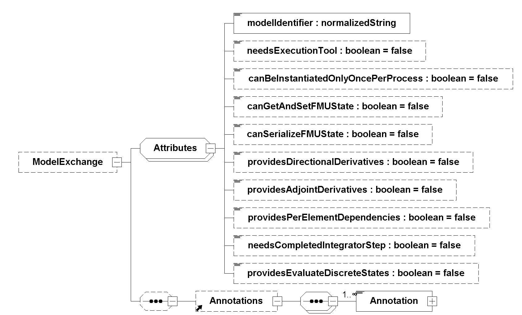
The attribute in the following table is defined in addition to the common attributes and has the following meaning (all attributes are optional with exception of modelIdentifier):
| Attribute | Description |
|---|---|
|
If |
3.4.1. Example Model Description File
When generating an FMU from the hypothetical model MyLibrary.SpringMassDamper, the XML file may have the following content:
<?xml version="1.0" encoding="UTF-8"?>
<fmiModelDescription
  fmiVersion="3.0"
  modelName="MyLibrary.SpringMassDamper"
  instantiationToken="{8c4e810f-3df3-4a00-8276-176fa3c9f9e0}"
  description="Rotational Spring Mass Damper System"
  version="1.0"
  generationDateAndTime="2022-05-01T16:57:33Z"
  variableNamingConvention="structured">
  <ModelExchange modelIdentifier="MyLibrary_SpringMassDamper"/>
  <UnitDefinitions>
    <Unit name="rad">
      <BaseUnit rad="1"/>
      <DisplayUnit name="deg" factor="57.2957795130823"/>
    </Unit>
    <Unit name="rad/s">
      <BaseUnit s="-1" rad="1"/>
    </Unit>
    <Unit name="kg.m2">
      <BaseUnit kg="1" m="2"/>
    </Unit>
    <Unit name="N.m">
      <BaseUnit kg="1" m="2" s="-2"/>
    </Unit>
  </UnitDefinitions>
  <TypeDefinitions>
    <Float64Type name="Modelica.Units.SI.Inertia" quantity="MomentOfInertia" unit="kg.m2" min="0.0"/>
    <Float64Type name="Modelica.Units.SI.Torque" quantity="Torque" unit="N.m"/>
    <Float64Type name="Modelica.Units.SI.AngularVelocity" quantity="AngularVelocity" unit="rad/s"/>
    <Float64Type name="Modelica.Units.SI.Angle" quantity="Angle" unit="rad"/>
  </TypeDefinitions>
  <DefaultExperiment startTime="0.0" stopTime="3.0" tolerance="0.0001"/>
  <ModelVariables>
    <Float64 name="inertia1.J" valueReference="1073741824"
      description="Moment of load inertia" causality="parameter" variability="fixed"
      declaredType="Modelica.Units.SI.Inertia" start="1"/>
    <Float64 name="torque.tau" valueReference="536870912"
      description="Accelerating torque acting at flange (= -flange.tau)" causality="input"
      declaredType="Modelica.Units.SI.Torque" start="0"/>
    <Float64 name="inertia1.phi" valueReference="805306368"
      description="Absolute rotation angle of component" causality="output"
      declaredType="Modelica.Units.SI.Angle"/>
    <Float64 name="inertia1.w" valueReference="805306369"
      description="Absolute angular velocity of component (= der(phi))" causality="output"
      declaredType="Modelica.Units.SI.AngularVelocity"/>
    <Float64 name="x[1]" valueReference="0" initial="exact" start="0"/>
    <Float64 name="x[2]" valueReference="1" initial="exact" start="0"/>
    <Float64 name="der(x[1])" valueReference="2" derivative="0"/>
    <Float64 name="der(x[2])" valueReference="3" derivative="1"/>
  </ModelVariables>
  <ModelStructure>
    <Output valueReference="805306368"/>
    <Output valueReference="805306369"/>
    <ContinuousStateDerivative valueReference="2"/>
    <ContinuousStateDerivative valueReference="3"/>
    <InitialUnknown valueReference="805306368"/>
    <InitialUnknown valueReference="805306369"/>
    <InitialUnknown valueReference="2" dependencies="0 536870912"/>
    <InitialUnknown valueReference="3" dependencies="0 1"/>
  </ModelStructure>
</fmiModelDescription>
4. FMI for Co-Simulation
FMI for Co-Simulation provides a standardized interface for execution of simulation models or tools in a co-simulation environment. In contrast to FMI for Model Exchange, a Co-Simulation FMU implements not only the model algorithm, but also the required solution method. The data exchange between FMUs is restricted to discrete communication points \(t_i\) (unless Intermediate Update Mode is used). In the time between two communication points (or between entering Intermediate Update Mode), the subsystem inside an FMU is solved independently by internal means. This leads to a delay for information "traveling through" the FMU, so there cannot be an immediate reaction (direct feedthrough) as in Initialization Mode, Event Mode or Continuous-Time Mode of Model Exchange. The co-simulation algorithm of the importer controls the data exchange and the synchronization between FMUs.
The co-simulation algorithm itself is not part of the FMI standard.
The co-simulation algorithm is responsible for:
-
advancing the overall simulation time,
-
exchange input and output data,
-
triggering of input clocks, and
-
handling events.
For FMI for Co-Simulation the co-simulation algorithm is shielded from how the FMU advances time internally. [For example, FMUs containing ODEs and implementing FMI for Co-Simulation require to include an ODE solver inside the FMU to internally advance time between the communication points. As another example, FMUs representing controller code, an internal scheduling algorithm can trigger computations at the correct time and order while advancing time to the next communication point.]
FMI for Co-Simulation enables the following features, allowing co-simulation algorithms of arbitrary sophistication:
-
variable or constant communication step sizes \(h_i\) (see
communicationStepSize), -
reject and repeat communication steps (see Section 2.2.7.4), e.g. with reduced communication step size or a different set of input values,
-
update inputs and retrieve outputs at intermediate points within a communication step (see Intermediate Update Mode),
-
return early from
fmi3DoStepat \(t \leq t_{i+1}\), because, for example, an event influencing the environment was detected by the FMU (see early return), -
dedicated Initialization Mode, which allows computation of consistent initial conditions over algebraic loops,
-
the ability of the FMU to provide
derivativesofoutputsw.r.t. time, to allow approximation techniques (Section 4.1.2), and -
the ability of the FMU to provide directional and adjoint derivatives.
Which of the features above are supported by a specific FMU is defined by capability flags.
4.1. Concepts
4.1.1. Smoothness, Continuity and Discontinuity
Since inputs are set at specific communication points by the importer, the FMU must make assumptions about the values between these communication points, including points of intermediate updates.
Between communication points, even in Intermediate Update Mode, all changes must be assumed to be continuous.
Changes to continuous variables are only considered discrete in Event Mode.
If a continuous input changes discontinuously (e.g. the actual input value deviates too much from the extrapolation polynomial), the co-simulation algorithm of the importer must raise an event (if supported) to indicate to the FMU a discontinuous change of a continuous input.
In the case of Co-Simulation without Event Mode (see eventModeUsed and hasEventMode), detecting discrete changes to continuous input variables (for instance to reset the integration algorithm within the FMU) requires heuristics.
4.1.2. Getting Derivatives of Continuous Outputs
In FMI for Co-Simulation, the n-th derivatives with respect to time of continuous outputs may be retrieved with fmi3GetOutputDerivatives, for example, to allow interpolation/extrapolation of connected input variables between communication points by the importer.
Whether the FMU is able to provide the derivatives of outputs is given by the capability flag maxOutputDerivativeOrder that represents the maximum order of the output derivatives.
If the actual order is lower (because the order of integration algorithm is low), the retrieved value is 0.
The returned values correspond to the derivatives at the current time of the FMU.
For example, after a successful call to fmi3DoStep, the returned values are related to the end of the communication step.
- Function
fmi3GetOutputDerivatives
typedef fmi3Status fmi3GetOutputDerivativesTYPE(fmi3Instance instance,
                                                const fmi3ValueReference valueReferences[],
                                                size_t nValueReferences,
                                                const fmi3Int32 orders[],
                                                fmi3Float64 values[],
size_t nValues);-
valueReferencesis a vector of value references that define the variables whosederivativesshall be retrieved. If multiple derivatives of a variable shall be retrieved, list the value reference multiple times. -
nValueReferencesis the dimension of the argumentsvalueReferencesandorders. -
orderscontains the orders of the respectivederivative(1 means the firstderivative, 2 means the secondderivative, …, 0 is not allowed). If multiple derivatives of a variable shall be retrieved, its value reference must occur multiple times invalueReferencesaligned with the correspondingordersarray. -
valuesis a vector with the values of thederivatives. The order of thevalueselements is derived from a twofold serialization: the outer level corresponds to the combination of a value reference (e.g.,valueReferences[k]) and order (e.g.,orders[k]), and the inner level to the serialization of variables as defined in Section 2.2.7.1. The inner level does not exist for scalar variables. -
nValuesis the size of the argumentvalues.nValuesonly equalsnValueReferencesif all corresponding output variables are scalar variables.
[ Example:
Assuming an FMU has outputs \(y_1\)[2x3] with value reference 1, \(y_2\) with value reference 2, \( y_3\)[2] value reference 3, \(y_4\) with value reference 4 and maxOutputDerivativeOrder = 2.
With valueReferences = [1, 1, 3, 3, 4, 4], and orders = [1, 2, 1, 2, 1, 2], fmi3GetOutputDerivatives will provide first and second time derivatives of the outputs y1, y3, y4, which in values are serialized in the following way:
((array serialization of \(\dot y_1\)), (array serialization of \(\ddot y_1\)), (array serialization of \(\dot y_3\)), (array serialization of \(\ddot y_3\)), \(\dot y_4\), \(\ddot y_4\)).]
4.1.3. Early Return
A Co-Simulation FMU is allowed to stop the execution of fmi3DoStep and return without reaching the predefined communication time, i.e. currentCommunicationPoint + communicationStepSize.
This mechanism is called "early return".
Early return can be used to shorten a communication step because of:
-
an event happened inside the FMU which influences its outputs non-continuously.
-
the importer requests the stop of the current communication step in Intermediate Update Mode. [E.g. the importer wants to stop a communication step because other parts of the simulation indicate the necessity.]
-
the FMU requests an additional communication point. [E.g. the FMU wants to communicate extrema of outputs or prevent model inconsistencies, like negative pressure values, caused by extrapolation of inputs.]
For details see the argument earlyReturn of fmi3DoStep.
The capability flag canReturnEarlyAfterIntermediateUpdate describes if the FMU supports early return after Intermediate Update Mode if requested by the importer.
The argument earlyReturnAllowed of fmi3InstantiateCoSimulation signals to the FMU if the importer allows early return.
4.2. State Machine for Co-Simulation
The state machine in Figure 42 defines the allowed calling sequences for FMI for Co-Simulation.

Common states are defined in Section 2.3, such as super states FMU State Settable and Initialized, states Instantiated, Configuration Mode, Reconfiguration Mode, Initialization Mode, Event Mode, and Terminated.
4.2.1. State: Step Mode
The state Step Mode is used to compute the values of all variables between communication points and events and to advance time in the FMU.
If the FMU is connected in algebraic loops with other models, iterations over the FMU equations requires setting the FMU to a state previously stored (using fmi3GetFMUState and fmi3SetFMUState) and repeating fmi3DoStep.
During Step Mode, clocked variables can not be set or get because Clocks are only active during Event Mode.
| Equations and Actions | Functions Influencing Equations |
|---|---|
Set |
|
Set non-clocked, continuous-time and discrete-time |
|
Get values of non-clocked variables \(\mathbf{v}_{-k}(t)\). |
|
Get time derivatives of |
|
|
|
\((\mathbf{v}_{u-k}, t_u) := \mathbf{f}_{\mathit{inter}}({}^{\bullet}\mathbf{x}_d, \mathbf{u}_{c+d}, {}^{\bullet}\mathbf{u}_{\mathit{c,u}}, \mathbf{p}, {}^{\bullet}\mathbf{b}, t_i, h_i)\) |
|
Activate event equations \(\mathbf{f}_{\mathit{event}}\). |
- Allowed Function Calls
- Function
fmi3Set{VariableType} -
sets the values of variables with:
at time \(t\).
- Function
fmi3Get{VariableType} -
returns values for all variables at \(t\).
fmi3Get{VariableType}does not trigger an evaluation of \(\mathbf{f}_{\mathit{doStep}}\). Therefore, algebraic loops at communication points cannot be handled by an appropriate sequence offmi3Get{VariableType}andfmi3Set{VariableType}calls [contrary to Initialization Mode, Event Mode and Continuous-Time Mode]. Repeating a communication step requires to reset the FMU state to the previous communication point withfmi3SetFMUStateand repeating thefmi3DoStepwith new input values.Calling
fmi3Get{VariableType}is not allowed afterfmi3Set{VariableType}without callingfmi3DoStepin between. [This allows for more efficient FMU implementations that avoid double buffering and allows in-place operations.] - Function
fmi3GetOutputDerivatives -
See Section 4.1.2.
- Function
fmi3GetDirectionalDerivative - Function
fmi3GetAdjointDerivative - Function
fmi3DoStep -
The importer requests the computation of the next time step with the following function:
typedef fmi3Status fmi3DoStepTYPE(fmi3Instance instance,
                                  fmi3Float64 currentCommunicationPoint,
                                  fmi3Float64 communicationStepSize,
                                  fmi3Boolean noSetFMUStatePriorToCurrentPoint,
                                  fmi3Boolean* eventHandlingNeeded,
                                  fmi3Boolean* terminateSimulation,
                                  fmi3Boolean* earlyReturn,
                                  fmi3Float64* lastSuccessfulTime);
Only
fmi3DoStepcan change the time of a Co-Simulation FMU from the outside (time advances internally duringfmi3DoStep). Arguments referring to time inherit the unit of theindependentvariable.-
currentCommunicationPointis the current communication point of the importer (\(t_{i}\)). At the first call offmi3DoStep,currentCommunicationPointmust be equal to the argumentstartTimeoffmi3EnterInitializationMode. -
communicationStepSizeis the communication step size (\(h_{i}\)).communicationStepSizemust be \(> 0.0\). The FMU is expected to compute until time \(t_{i+1} = t_{i} + h_{i}\). SeecanHandleVariableCommunicationStepSizefor restrictions.[Formally, argument
currentCommunicationPointis not needed. It is present in order to handle a potential mismatch between the importer’s and the FMU’s time representations and/or computations. Both argumentscurrentCommunicationPointandcommunicationStepSizeallow computing of \(t_{i+1}\) by one addition, avoiding accumulation of numerical errors.] -
noSetFMUStatePriorToCurrentPoint = fmi3Trueiffmi3SetFMUStatewill no longer be called for time instants prior tocurrentCommunicationPointin this simulation run.[The FMU can use this flag to flush a result buffer.]
-
eventHandlingNeeded = fmi3Trueindicates that an event was encountered by the FMU atlastSuccessfulTimeand the importer has to enter Event Mode by callingfmi3EnterEventMode.eventHandlingNeeded = fmi3Truemust not be signaled, if the importer indicates to not support Event Mode byeventModeUsed = fmi3False. [This is different fromearlyReturnwhich only indicates that thefmi3DoStepdid not complete the intended step up untilcurrentCommunicationPoint+communicationStepSizeand does not require event handling.] -
When
terminateSimulation = fmi3True, the FMU requests to stop the simulation and the importer must callfmi3Terminate. -
earlyReturnsignals to the importer that the FMU returns at \(t_{i+1} < t_i +\)communicationStepSize.earlyReturn = fmi3Trueis only allowed ifearlyReturnAllowed = fmi3Trueinfmi3InstantiateCoSimulation. The time reached is specified inlastSuccessfulTime. Reasons forearlyReturn = fmi3Trueare-
expressed by the return arguments
eventHandlingNeededorterminateSimulationoffmi3DoStep, or -
the FMU’s reaction to the importers request for
earlyReturnby the return argumentearlyReturnRequested = fmi3Trueoffmi3IntermediateUpdateCallback, or -
the FMU’s request for a communication point at
lastSuccessfulTimefor any other reason.
-
-
lastSuccessfulTimerepresents the internal time \(t_{i+1}\) of the FMU whenfmi3DoStepreturns, for any value ofearlyReturn. It is possible that thelastSuccessfulTimeis equal tocurrentCommunicationPointwhenearlyReturn = fmi3Trueto indicate, for example, the detection of an event atcurrentCommunicationPoint. Even if the FMU returns fromfmi3DoStepwithfmi3OKandearlyReturn = fmi3False, it is allowed thatlastSuccessfulTimedeviates from the expectedcurrentCommunicationPoint+communicationStepSize. [Examples:-
A fixed-step integrator inside the FMU cannot reach the requested time exactly.
fixedInternalStepSizewas introduced to counter these effects. -
A variable-step integrator with minimal step size is not able to land exactly at \(t_{i+1}\).]
-
-
- Function
fmi3IntermediateUpdateCallback -
fmi3IntermediateUpdateCallbackswitches the FMU itself into the Intermediate Update Mode.
- Function
fmi3EnterEventMode -
typedef fmi3Status fmi3EnterEventModeTYPE(fmi3Instance instance);This function changes the state to Event Mode.
The importer must call
fmi3EnterEventModewhen any of the following conditions are met:-
time has reached
nextEventTimeas returned byfmi3UpdateDiscreteStates, or -
the FMU returned with eventHandlingNeeded = fmi3True from
fmi3DoStep, or -
the importer plans discrete changes to inputs, or
-
an input Clock needs to be set.
This function must not be called, if
fmi3InstantiateCoSimulationsignaledeventModeUsed = fmi3False, which can be forced by the FMU withhasEventMode = false. -
- Function
fmi3EnterConfigurationMode -
fmi3EnterConfigurationModechanges state to Reconfiguration Mode.fmi3EnterConfigurationModemust not be called if the FMU contains notunablestructural parameters(i.e. withcausality=structuralParameterandvariability=tunable).
4.2.2. State: Intermediate Update Mode
Intermediate Update Mode can only be entered by the FMU itself using the callback function fmi3IntermediateUpdateCallback.
An FMU may enter Intermediate Update Mode in order to exchange input and output values between communication points.
Furthermore, the Intermediate Update Mode allows the importer to request an early return from the current fmi3DoStep because of an event between communication points.
The importer cannot request entering Intermediate Update Mode from the FMU and hence for some use cases (e.g. cooperative multitasking and setting of intermediate input values) the importer relies on the callbacks from the FMUs.
Intermediate Update Mode enables:
-
enables advanced Co-Simulation with interpolation/extrapolation techniques of inputs and outputs (such as polynomial extrapolation, Transmission Line Modeling (TLM) co-simulation, anti-alias filtering, smoothing of input among others).
-
the same input approximation that was possible in FMI 2.0 with
fmi2SetInputDerivatives, by evaluation of the approximation polynomial by the importer and not within the FMU as in FMI 2.0.
The FMU signals the support of Intermediate Update Mode via the capability flag providesIntermediateUpdate.
The co-simulation algorithm signals the support for Intermediate Update Mode by providing a non-NULL callback-function pointer for intermediateUpdate.
Intermediate values for continuous inputs are computed by the importer for example by an extrapolation polynomial build with the output derivatives of connected FMUs.
FMUs can signal with the optional attribute recommendedIntermediateInputSmoothness of value \(k\) to the co-simulation algorithm that best convergence rates can be achieved if these approximation functions are of smoothness \(C^{k}([t_i, t_{i+1}])\), that is k-time continuously differentiable, with \(C^{0}\) meaning continuous.
[This can increase simulation speed for higher order multi-step solvers that in this case do not have to reset at communication points.]
The importer must ensure that the input approximation function \(\mathbf{u}_u\) is consistent with the values of the input variable (\(\mathbf{u}_u(t_{i+1})= \mathbf{u}(t_{i+1})\)).
Due to the way FMU internal solvers may estimate and correct the approximation error, tentative states may occur and lead to tentative intermediate output values (see intermediateStepFinished).
If an FMU internal integration step has been completed successfully, the importer can forward intermediate outputs to other FMUs, where they can be used to approximate inputs.
Figure 43 summarizes the above description. It illustrates multiple intermediate internal solver steps, distinguishing between the final ones (with black-filled circles) and tentative ones (with white-filled circles). It distinguishes the level of trust that can be placed in the tentative outputs (with dashed arrows) and in final outputs (with solid arrows).

The FMU enters Intermediate Update Mode by calling fmi3IntermediateUpdateCallback within Step Mode and leaves the state towards Step Mode when the function returns.
typedef void (*fmi3IntermediateUpdateCallback) (
    fmi3InstanceEnvironment instanceEnvironment,
    fmi3Float64  intermediateUpdateTime,
    fmi3Boolean  intermediateVariableSetRequested,
    fmi3Boolean  intermediateVariableGetAllowed,
    fmi3Boolean  intermediateStepFinished,
    fmi3Boolean  canReturnEarly,
    fmi3Boolean* earlyReturnRequested,
fmi3Float64* earlyReturnTime);-
intermediateUpdateTimeis the internal value of theindependentvariable [typically simulation time] of the FMU at which the callback has been called.intermediateUpdateTimeis restricted by the arguments offmi3DoStepas follows:
currentCommunicationPoint\(\leq\)intermediateUpdateTime\(\leq\) (currentCommunicationPoint+communicationStepSize).
The FMU must not call the callback functionfmi3IntermediateUpdateCallbackwith anintermediateUpdateTimethat is smaller than theintermediateUpdateTimegiven in a previous call offmi3IntermediateUpdateCallbackwithintermediateStepFinished = fmi3True.
-
If
intermediateVariableSetRequested = fmi3True, the importer may provide intermediate values for continuousinputvariables withintermediateUpdate = trueby callingfmi3Set{VariableType}. The set of variables for which the importer may provide intermediate values is declared through therequiredIntermediateVariablesargument offmi3InstantiateCoSimulation. If the importer does not provide a new value for any of the variables contained in the set it registered, the values set last remain.
-
If
intermediateVariableGetAllowed = fmi3True, the importer may obtain intermediate output values by callingfmi3Get{VariableType}for variables withintermediateUpdate = true. The set of variables for which the importer may get values is defined by therequiredIntermediateVariablesargument offmi3InstantiateCoSimulation.
-
If
intermediateStepFinished = fmi3False, the intermediate output values of the FMU that the importer inquires withfmi3Get{VariableType}resulting from tentative internal solver states and may still change for the sameintermediateUpdateTime[e.g., if the solver deems the tentative state to cause an unacceptable approximation error, it may go back in time and try to re-estimate the state using smaller internal time steps].
IfintermediateStepFinished = fmi3True, intermediate output values inquired by the importer withfmi3Get{VariableType}correspond to accepted internal solver steps.
-
When
canReturnEarly = fmi3Truethe FMU signals to the importer its ability to return early from the currentfmi3DoStep.
-
earlyReturnRequested: If and only ifcanReturnEarly = fmi3True, the importer may request the FMU to return early fromfmi3DoStepby settingearlyReturnRequested = fmi3True.
-
earlyReturnTimeis used to signal the FMU at which time to return early from the currentfmi3DoStep, ifearlyReturnRequested = fmi3True. If theearlyReturnTimeis greater than the currentintermediateUpdateTime, the FMU may compute up toearlyReturnTime.earlyReturnTimeis restricted by the arguments offmi3DoStepas follows:
currentCommunicationPoint\(\leq\)earlyReturnTime\(\leq\) (currentCommunicationPoint+communicationStepSize).
| Equations and Actions | Functions Influencing Equations |
|---|---|
Get intermediate variable values \(\mathbf{v}_u(t_u)\) |
|
Get time derivatives of |
|
Set continuous intermediate input variables \(\mathbf{u}_{\mathit{c,u}}(t_u)\) |
- Allowed Function Calls
- Function
fmi3Get{VariableType} -
This function can be called for intermediate variables, if
intermediateVariableGetAllowed = fmi3True. Intermediate variables are variables that are marked with attributeintermediateUpdate = truein themodelDescription.xmland have been included in therequiredIntermediateVariablesargument offmi3InstantiateCoSimulation. - Function
fmi3GetOutputDerivatives -
For details on
fmi3GetOutputDerivativessee Section 4.1.2. Furthermore, callingfmi3GetOutputDerivativesis only allowed on variables as defined forfmi3Get{VariableType}above. - Function
fmi3Set{VariableType} -
This function can be called for intermediate input variables, if
intermediateVariableSetRequested = fmi3True. Intermediate input variables are input variables that are marked with attributeintermediateUpdate = truein themodelDescription.xmland have been included in therequiredIntermediateVariablesargument offmi3InstantiateCoSimulation. Discreteinputsmust not be set.
There is a defined order of calling these functions: first all fmi3Get{VariableType} calls must be performed, then fmi3Set{VariableType} may be called.
[This is analogous to the calling sequence of fmi3Get{VariableType} and fmi3Set{VariableType} calls in Step Mode.]
4.3. Code Examples
4.3.1. Basic Co-Simulation
    CALL(FMI3InstantiateCoSimulation(S,
        INSTANTIATION_TOKEN, // instantiationToken
        resourcePath(),      // resourcePath
        fmi3False,           // visible
        fmi3False,           // loggingOn
        fmi3False,           // eventModeUsed
        fmi3False,           // earlyReturnAllowed
        NULL,                // requiredIntermediateVariables
        0,                   // nRequiredIntermediateVariables
        NULL                 // intermediateUpdate
    ));

    // set start values
    CALL(applyStartValues(S));

    // initialize the FMU
    CALL(FMI3EnterInitializationMode(S, fmi3False, 0.0, startTime, fmi3True, stopTime));

    CALL(FMI3ExitInitializationMode(S));

    for (int step = 0;; step++) {

        CALL(recordVariables(S, outputFile));

        // calculate the current time
        const fmi3Float64 time = step * h;

        CALL(applyContinuousInputs(S, false));
        CALL(applyDiscreteInputs(S));

        if (time >= stopTime) {
            break;
        }

        // call instance s1 and check status
        CALL(FMI3DoStep(S, time, h, fmi3True, &eventEncountered, &terminateSimulation, &earlyReturn, &lastSuccessfulTime));

        if (terminateSimulation) {
            printf("The FMU requested to terminate the simulation.");
            break;
        }
    }

TERMINATE:
    return tearDown();
The plot below shows the output for the BouncingBall Reference FMU with a communication step size of 0.1 s. Note that the points where the ball hits the floor are missed.

4.3.2. Early Return
    CALL(FMI3InstantiateCoSimulation(S,
        INSTANTIATION_TOKEN, // instantiationToken
        NULL,                // resourcePath
        fmi3False,           // visible
        fmi3False,           // loggingOn
        fmi3False,           // eventModeUsed
        fmi3True,            // earlyReturnAllowed
        NULL,                // requiredIntermediateVariables
        0,                   // nRequiredIntermediateVariables
        NULL                 // intermediateUpdate
    ));

    // set start values
    CALL(applyStartValues(S));

    fmi3Float64 time = startTime;

    // initialize the FMU
    CALL(FMI3EnterInitializationMode(S, fmi3False, 0.0, time, fmi3True, stopTime));

    CALL(FMI3ExitInitializationMode(S));

    // communication step size
    const fmi3Float64 stepSize = 10 * FIXED_SOLVER_STEP;

    while (true) {

        // apply continuous and discrete inputs
        CALL(applyContinuousInputs(S, true));
        CALL(applyDiscreteInputs(S));

        // record variables
        CALL(recordVariables(S, outputFile));

        if (terminateSimulation || time >= stopTime) {
            break;
        }

        // returns early on events
        CALL(FMI3DoStep(S,
            time,                 // currentCommunicationPoint
            stepSize,             // communicationStepSize
            fmi3True,             // noSetFMUStatePriorToCurrentPoint
            &eventEncountered,    // eventEncountered
            &terminateSimulation, // terminate
            &earlyReturn,         // earlyReturn
            &time                 // lastSuccessfulTime
        ));
    }

TERMINATE:
    return tearDown();
The plot below shows the output for the BouncingBall Reference FMU with a communication step size of 0.1 s. Note that the points where the ball hits the floor are available, but only the outputs after the events are recorded.

4.3.3. Event Mode
    CALL(FMI3InstantiateCoSimulation(S,
        INSTANTIATION_TOKEN, // instantiationToken
        NULL,                // resourcePath
        fmi3False,           // visible
        fmi3False,           // loggingOn
        fmi3True,            // eventModeUsed
        fmi3True,            // earlyReturnAllowed
        NULL,                // requiredIntermediateVariables
        0,                   // nRequiredIntermediateVariables
        NULL                 // intermediateUpdate
    ));

    // set start values
    CALL(applyStartValues(S));

    fmi3Float64 time = startTime;

    // initialize the FMU
    CALL(FMI3EnterInitializationMode(S, fmi3False, 0.0, time, fmi3True, stopTime));

    // apply continuous and discrete inputs
    CALL(applyContinuousInputs(S, true));
    CALL(applyDiscreteInputs(S));

    CALL(FMI3ExitInitializationMode(S));

    // update discrete states
    do {
        CALL(FMI3UpdateDiscreteStates(S,
            &discreteStatesNeedUpdate,
            &terminateSimulation,
            &nominalsChanged,
            &statesChanged,
            &nextEventTimeDefined,
            &nextEventTime
        ));

        if (terminateSimulation) {
            goto TERMINATE;
        }
    } while (discreteStatesNeedUpdate);

    CALL(FMI3EnterStepMode(S));

    // communication step size
    const fmi3Float64 stepSize = 10 * FIXED_SOLVER_STEP;

    while (true) {

        CALL(recordVariables(S, outputFile));

        if (terminateSimulation || time >= stopTime) {
            break;
        }

        CALL(FMI3DoStep(S,
            time,                 // currentCommunicationPoint
            stepSize,             // communicationStepSize
            fmi3True,             // noSetFMUStatePriorToCurrentPoint
            &eventEncountered,    // eventEncountered
            &terminateSimulation, // terminate
            &earlyReturn,         // earlyReturn
            &time                 // lastSuccessfulTime
        ));

        if (eventEncountered) {

            // record variables before event update
            CALL(recordVariables(S, outputFile));

            // enter Event Mode
            CALL(FMI3EnterEventMode(S));

            // apply continuous and discrete inputs
            CALL(applyContinuousInputs(S, true));
            CALL(applyDiscreteInputs(S));

            // update discrete states
            do {
                CALL(FMI3UpdateDiscreteStates(S,
                    &discreteStatesNeedUpdate,
                    &terminateSimulation,
                    &nominalsChanged,
                    &statesChanged,
                    &nextEventTimeDefined,
                    &nextEventTime
                ));

                if (terminateSimulation) {
                    break;
                }
            } while (discreteStatesNeedUpdate);

            // return to Step Mode
            CALL(FMI3EnterStepMode(S));
        }
    }

TERMINATE:
    return tearDown();
The plot below shows the output for the BouncingBall Reference FMU with a communication step size of 0.1 s. Note that the points where the ball hits the floor are available and the outputs before and after the event are recorded.

4.3.4. Intermediate Update
void intermediateUpdate(fmi3InstanceEnvironment instanceEnvironment,
                           fmi3Float64 intermediateUpdateTime,
                           fmi3Boolean intermediateVariableSetRequested,
                           fmi3Boolean intermediateVariableGetAllowed,
                           fmi3Boolean intermediateStepFinished,
                           fmi3Boolean canReturnEarly,
                           fmi3Boolean *earlyReturnRequested,
                           fmi3Float64 *earlyReturnTime) {

    if (!instanceEnvironment) {
        return;
    }

    FMIInstance *S = (FMIInstance *)instanceEnvironment;

    S->time = intermediateUpdateTime;

    *earlyReturnRequested = fmi3False;
    *earlyReturnTime = 0;

    // if getting intermediate output variables is allowed
    if (intermediateVariableGetAllowed) {

        // Get the output variables at time == intermediateUpdateTime
        // fmi3Get{VariableType}();
        status = recordVariables(S, outputFile);

        // If integration step in FMU solver is finished
        if (intermediateStepFinished) {
            //Forward output variables to other FMUs or write to result files
        }
    }

    // if setting intermediate output variables is allowed
    if (intermediateVariableSetRequested) {
        // Compute intermediate input variables from output variables and
        // variables from other FMUs. Use latest available output
        // variables, possibly from get functions above.
        // inputVariables = ...

        // Set the input variables at time == intermediateUpdateTime
        // fmi3Set{VariableType}();
    }

    // Internal execution in FMU will now continue

    // TODO: handle status

    // log function call
    fprintf(logFile, "intermediateUpdate("
        "instanceEnvironment=0x%p, "
        "intermediateUpdateTime=%.16g, "
        "intermediateVariableSetRequested=%d, "
        "intermediateVariableGetAllowed=%d, "
        "intermediateStepFinished=%d, "
        "canReturnEarly=%d, "
        "earlyReturnRequested=%d, "
        "earlyReturnTime=%.16g)\n",
        instanceEnvironment,
        intermediateUpdateTime,
        intermediateVariableSetRequested,
        intermediateVariableGetAllowed,
        intermediateStepFinished,
        canReturnEarly,
        *earlyReturnRequested,
        *earlyReturnTime
    );
}
The plot below shows the output for the BouncingBall Reference FMU with a communication step size of 0.1 s. Note that the outputs at all intermediate steps are recorded, too.

4.3.5. Connected FMUs
In the following example, the usage of the FMI functions is sketched in order to clarify the typical calling sequence of the functions in a simulation environment.
We consider two FMUs, where both have one continuous floating point input and one continuous floating point output which are connected in the following way:

We assume no algebraic dependency between input and output of each FMU.
The code demonstrates the simplest importer as shown in Section 4.2:
-
Constant communication step size.
-
No repeating of communication steps.
-
The error handling is implemented in a very rudimentary way.
////////////////////////////
// Initialization sub-phase
typedef fmi3Instance fmi3InstantiateCoSimulationTYPE(
    fmi3String                     instanceName,
    fmi3String                     instantiationToken,
    fmi3String                     resourceLocation,
    fmi3Boolean                    visible,
    fmi3Boolean                    loggingOn,
    fmi3Boolean                    eventModeUsed,
    fmi3Boolean                    earlyReturnAllowed,
    const fmi3ValueReference       requiredIntermediateVariables[],
    size_t                         nRequiredIntermediateVariables,
    fmi3InstanceEnvironment        instanceEnvironment,
    fmi3CallbackLogMessage         logMessage,
    fmi3CallbackIntermediateUpdate intermediateUpdate);

// instantiate both FMUs
s1 = s1_fmi3InstantiateCoSimulation("s1",          // instanceName
                                    guid,          // instantiationToken
                                    NULL,          // resourceLocation
                                    fmi3False,     // visible
                                    fmi3False,     // loggingOn
                                    fmi3False,     // eventModeUsed
                                    fmi3False,     // earlyReturnAllowed
                                    NULL,          // requiredIntermediateVariables
                                    0,             // nRequiredIntermediateVariables
                                    NULL,          // instanceEnvironment
                                    cb_logMessage, // logMessage
                                    NULL);         // intermediateUpdate

s2 = s2_fmi3InstantiateCoSimulation("s2",          // instanceName
                                    guid,          // instantiationToken
                                    NULL,          // resourceLocation
                                    fmi3False,     // visible
                                    fmi3False,     // loggingOn
                                    fmi3False,     // eventModeUsed
                                    fmi3False,     // earlyReturnAllowed
                                    NULL,          // requiredIntermediateVariables
                                    0,             // nRequiredIntermediateVariables
                                    NULL,          // instanceEnvironment
                                    cb_logMessage, // logMessage
                                    NULL);         // intermediateUpdate

if (s1 == NULL || s2 == NULL)
    return EXIT_FAILURE;

// start and stop time
startTime = 0;
stopTime = 10;

// communication step size
h = 0.01;

// set all variable start values (of "ScalarVariable / <type> / start")
// s1_fmi3Set{VariableType}(s1, ...);
// s2_fmi3Set{VariableType}(s2, ...);

// initialize the FMUs
s1_fmi3EnterInitializationMode(s1, fmi3False, 0.0, startTime, fmi3True, stopTime);
s2_fmi3EnterInitializationMode(s2, fmi3False, 0.0, startTime, fmi3True, stopTime);

// set the input values at time = startTime
// fmi3Set{VariableType}(s1, ...);
// fmi3Set{VariableType}(s2, ...);

s1_fmi3ExitInitializationMode(s1);
s2_fmi3ExitInitializationMode(s2);

////////////////////////
// Simulation sub-phase
tc = startTime; // current time

while ((tc < stopTime) && (status == fmi3OK)) {

    // retrieve outputs
    // fmi3Get{VariableType}(s1, ..., 1, &y1);
    // fmi3Get{VariableType}(s2, ..., 1, &y2);

    // set inputs
    // fmi3Set{VariableType}(s1, ..., 1, &y2);
    // fmi3Set{VariableType}(s2, ..., 1, &y1);

    // call instance s1 and check status
    fmi3Boolean eventEncountered, terminateSimulation, earlyReturn;
    fmi3Float64 lastSuccessfulTime;

    status = s1_fmi3DoStep(s1, tc, h, fmi3True, &eventEncountered, &terminateSimulation, &earlyReturn, &lastSuccessfulTime);

    if (terminateSimulation) {
        printf("Instance s1 requested to terminate simulation.");
        break;
    }

    // call instance s2 and check status as above
    status = s2_fmi3DoStep(s2, tc, h, fmi3True, &eventEncountered, &terminateSimulation, &earlyReturn, &lastSuccessfulTime);

    // ...

    // increment current time
    tc += h;
 }

//////////////////////////
// Shutdown sub-phase
if (status != fmi3Error && status != fmi3Fatal) {
    s1_fmi3Terminate(s1);
    s2_fmi3Terminate(s2);
}

if (status != fmi3Fatal) {
    s1_fmi3FreeInstance(s1);
    s2_fmi3FreeInstance(s2);
}
4.4. Description Schema
XML elements and attributes common to all interface types are defined in FMI Description Schema.
Additional elements and attributes are defined subsequently.
If the FMU implements the Co-Simulation interface type, the element <CoSimulation> must be present.
It is defined as:
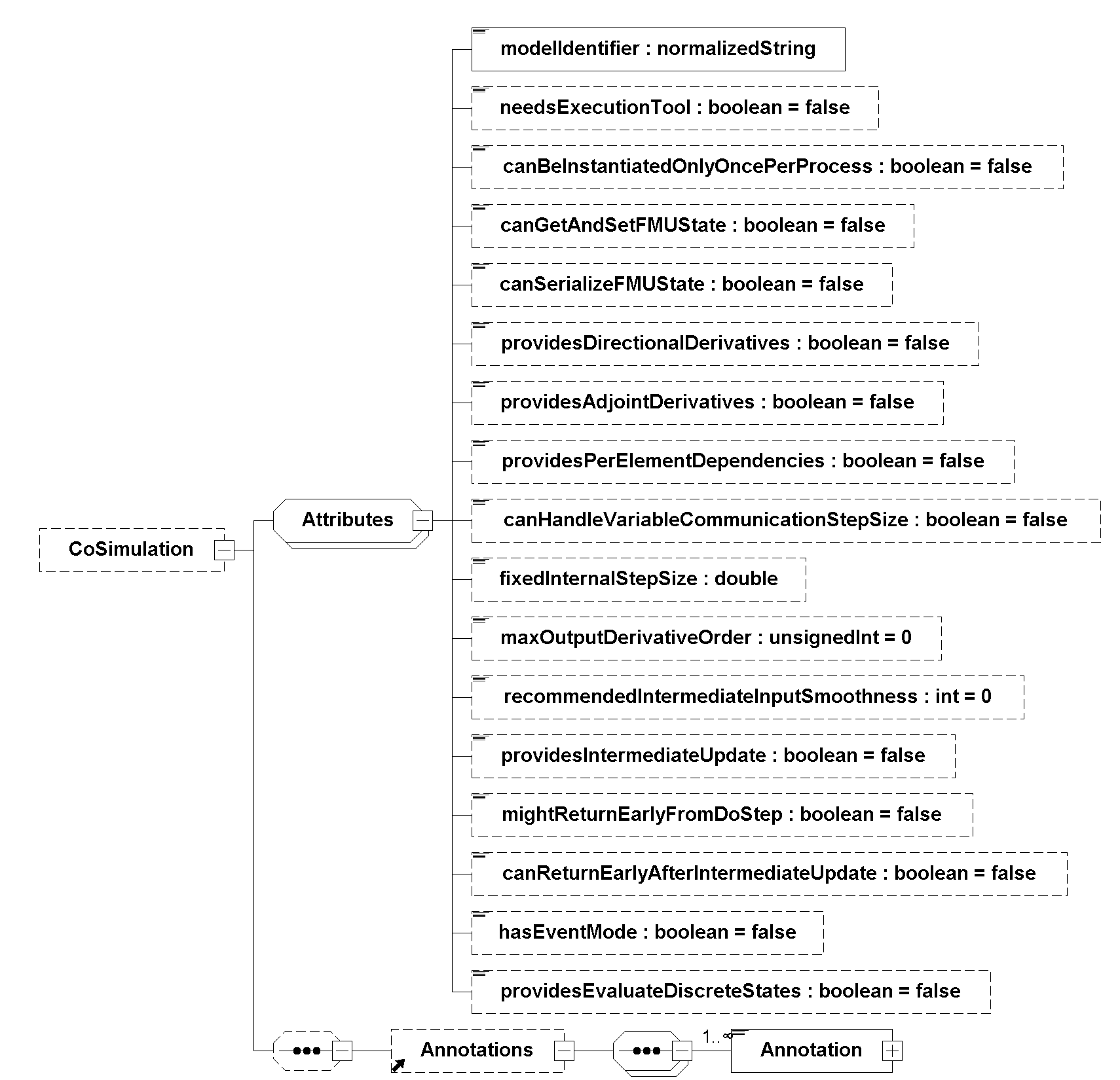
The attributes in the following table are defined in addition to the common attributes and have the following meaning (all attributes are optional with the exception of modelIdentifier):
| Attribute | Description |
|---|---|
|
If |
|
If the FMU has a fixed internal step size, this optional attribute communicates it. |
|
The FMU is able to provide |
|
A value of \(k\) with \(k>0\) signals to the importer, that it is beneficial for the solver within the FMU to receive intermediate inputs that are \(k\)-time continuously differentiable (\(C^k\)) on the current communication interval. \(k = 0\) means continuous (see Section 4.1.1). |
|
The FMU supports Intermediate Update Mode and will call |
|
The FMU announces that it might return early from |
|
If |
|
If |
4.4.1. Example Model Description File
4.4.1.1. Example Model Description File with Early Return
The Example <fmiModelDescription> below is the same as shown in Section 3.4.1 for a Model Exchange FMU.
The only differences are the replacement of the element <ModelExchange> with the element <CoSimulation> with additional Co-Simulation-specific attributes, and the removal of local variables, which are associated with continuous states and their derivatives.
<fmiModelDescription><?xml version="1.0" encoding="utf-8"?>
<fmiModelDescription
fmiVersion="3.0"
modelName="MyLibrary.SpringMassDamper_Early_Return_example"
instantiationToken="{8c4e810f-3df3-4a00-8276-176fa3c9f9e0}"
description="Rotational Spring Mass Damper System"
version="1.0"
generationDateAndTime="2022-05-01T16:57:33Z"
variableNamingConvention="structured">
<CoSimulation
modelIdentifier="MyLibrary_SpringMassDamper"
canHandleVariableCommunicationStepSize="true"
providesIntermediateUpdate="true"
canReturnEarlyAfterIntermediateUpdate="true"
hasEventMode="true"/>
<UnitDefinitions>
<Unit name="rad">
<BaseUnit rad="1"/>
<DisplayUnit name="deg" factor="57.2957795130823"/>
</Unit>
<Unit name="rad/s">
<BaseUnit s="-1" rad="1"/>
</Unit>
<Unit name="kg.m2">
<BaseUnit kg="1" m="2"/>
</Unit>
<Unit name="N.m">
<BaseUnit kg="1" m="2" s="-2"/>
</Unit>
</UnitDefinitions>
<TypeDefinitions>
<Float64Type name="Modelica.Units.SI.Inertia" quantity="MomentOfInertia" unit="kg.m2" min="0.0"/>
<Float64Type name="Modelica.Units.SI.Torque" quantity="Torque" unit="N.m"/>
<Float64Type name="Modelica.Units.SI.AngularVelocity" quantity="AngularVelocity" unit="rad/s"/>
<Float64Type name="Modelica.Units.SI.Angle" quantity="Angle" unit="rad"/>
</TypeDefinitions>
<DefaultExperiment startTime="0.0" stopTime="3.0" tolerance="0.0001"/>
<ModelVariables>
<Float64 name="inertia1.J" valueReference="1073741824"
description="Moment of load inertia" causality="parameter" variability="fixed"
declaredType="Modelica.Units.SI.Inertia" start="1"/>
<Float64 name="torque.tau" valueReference="536870912"
description="Accelerating torque acting at flange (= -flange.tau)" causality="input"
declaredType="Modelica.Units.SI.Torque" start="0"/>
<Float64 name="inertia1.phi" valueReference="805306368"
description="Absolute rotation angle of component" causality="output"
declaredType="Modelica.Units.SI.Angle"/>
<Float64 name="inertia1.w" valueReference="805306369"
description="Absolute angular velocity of component (= der(phi))" causality="output"
declaredType="Modelica.Units.SI.AngularVelocity"/>
</ModelVariables>
<ModelStructure>
<Output valueReference="805306368"/>
<Output valueReference="805306369"/>
<InitialUnknown valueReference="805306368"/>
<InitialUnknown valueReference="805306369"/>
</ModelStructure>
</fmiModelDescription>5. FMI for Scheduled Execution
The Scheduled Execution interface provides support for concurrent computation of model partitions on a single computational resource (e.g. CPU-core). The FMU exposes model partitions defined by its associated Clocks while the importer is enabled to explicitly schedule each model partition’s execution. As mentioned in Section 2.2.6, it is the importer respectively its scheduler that controls how time is progressing.
The following use cases and requirements motivate the introduction of this interface type:
-
The scheduler can execute a model partition at any time. It can execute model partitions periodically (either according to virtual time or real time) or reacting to an event, e.g. an event of an external I/O or an event sent from an FMU (see below).
-
The scheduler can run model partitions of one FMU together with model partitions of other FMUs or model partitions provided by other sources such as other models or functions in a single process.
-
The scheduler respects priorities of the model partitions defined by the FMU.
-
The Scheduled Execution interface allows the scheduler to preempt the execution of an FMU’s model partition. The importer is providing lock/unlock functions to the FMU to secure sections that should not be interrupted (e.g. the exchange of data between two model partitions of the same FMU).
-
The Scheduled Execution interface allows the FMU to send an event to the scheduler while a model partition is executed.
A parallel computation of model partitions is not part of the FMI 3.0 API. An FMU may still internally use parallel computation on multiple cores, but handling this is (currently) not part of the FMI standard.
5.1. Concepts
5.1.1. Activating Model Partitions
In Scheduled Execution the importer has to ensure that model partitions are scheduled according to their activation time and priorities.
This is realized in Clock Activation Mode by calling fmi3ActivateModelPartition triggering their respective Clocks.
The FMU may request to schedule another model partition even while currently a model partition is being executed.
In case more than one Clock ticks at the same time instant, the scheduler needs a priority to define the activation sequence of the associated model partitions.
This ordering is defined by the priority attributes of the Clock.
For Scheduled Execution this attribute is mandatory for every Clock.
[The Clock priorities are local to an FMU. It is not possible for an FMU exporting tool to know in advance the priorities of other FMUs that will be connected to an FMU in a simulation setup. It is the responsibility of the importer to derive a computational order for the computation of two or more distinct FMUs based on the local FMU Clock priorities and input-output relationships of connected FMUs.]
[For periodic Clocks it is recommended to derive the priorities based on a rate monotonic scheduling scheme (smallest period leads to highest priority, that is, has the smallest priority value.]
5.1.2. Preemption Support
If a model partition of lower priority is executed when a model partition of higher priority is activated, the scheduler must ensure that the execution of the latter one is not delayed and causing violations of timing constraints.
[On a real-time simulator a violation of a timing constraint usually results in an overrun exception i.e. a model partition is supposed to be executed when an instance of the same model partition has not yet finished its execution.]
Preemption support means that the scheduler can immediately interrupt the current execution of a model partition in order to execute a model partition of higher priority. The computation of the interrupted model partition is proceeded afterwards. So by regarding priorities and supporting preemption the scheduler can ensure that most critical model partitions are never delayed by less important model parts. [This is particularly important for real-time simulators as the wall clock time is dictating the time for the next execution.]
-
Same
priority: The scheduler does not preempt the execution of a model partition in favor of a model partition of the same priority. For model partitions with the same priority, the scheduler decides the execution order, e.g. based on configurations in the importer. -
Different priorities: The scheduler preempts the execution of a model partition of a lower priority as soon as a model partition of higher priority partition needs to be computed.
An example for scheduling based on priorities and preempting model partitions is given in section Section 5.3.
It may be important for the FMU to secure particular sections of its code against being preempted.
Callback functions fmi3LockPreemptionCallback and fmi3UnlockPreemptionCallback are provided by the importer when instantiating the FMU via fmi3InstantiateScheduledExecution to allow the FMU to signal entering and exiting such critical code sections.
typedef void (*fmi3LockPreemptionCallback)   ();
typedef void (*fmi3UnlockPreemptionCallback) ();
The FMU’s code has to be prepared to correctly handle preemption of
In general this means that the FMU’s code has to secure access to its global states and variables wherever data inconsistencies due to potential preemptions are anticipated.
[Note that depending on their implementation, fmi3CallbackLockPreemption and fmi3CallbackUnlockPreemption have a non-negligible overhead, as well as a strong impact on the scheduler and therefore their use should be as rare and short as possible.
In general it is recommended to reduce dependencies between different model partitions of one FMU by design.
In particular a unique assignment of the respective variables to model partitions via its associated Clock is strongly recommended.
One may also consider if the code can be preempted by other parts of the same FMU: E.g. a model partition cannot be interrupted if it is the only model partition or if it holds the highest priority. Similarly, a model partition, while it might be interrupted, might not need to guard data accesses if it is the only model partition of the FMU, or the one with the highest priority. In such cases no locks may be necessary.]
5.2. State Machine for Scheduled Execution
The state machine in Figure 46 defines the allowed calling sequences for FMI for Scheduled Execution.

Common states are defined in Section 2.3, such as super states FMU State Settable and Initialized, states Instantiated, Configuration Mode, Reconfiguration Mode, Initialization Mode, and Terminated.
State changes are global to all model partitions, except to and from Clock Update Mode.
E.g. if any function call returns fmi3Discard or fmi3Error, all active or preempted model partitions are in the same state.
In Scheduled Execution, fmi3Discard must be treated like fmi3Error.
If the simulation algorithm intends to enter the state Terminated, it must ensure that all function calls related to model partitions of the FMU have returned.
If in states Clock Activation Mode, Clock Update Mode, or Reconfiguration Mode a function returns fmi3Fatal, the importer may prematurely end all computations of model partitions of this FMU.
If in these states a function returns fmi3Discard or fmi3Error the importer may wait until all other model partitions of this FMU have ended, but new model partitions must not be started and all other function calls for this FMU must return fmi3Error until the state Terminated is reached.
5.2.1. State: Clock Activation Mode
In Clock Activation Mode the scheduler of the importer activates model partitions according to their respective Clock and priority definitions.
An FMU of type Schedule Execution exposes its provided model partitions by defining associated Clocks in its modelDescription.xml.
The scheduler must activate the model partitions by calling fmi3ActivateModelPartition (as well as related fmi3Get{VariableType} and fmi3Set{VariableType}) for each associated Clock, according to its properties, e.g. intervalDecimal and priority.
By scheduling the exposed model partitions of an FMU and executing them at dedicated points in time it is the scheduler that defines how time progresses, see Section 2.2.6.
The current time \(t_i\) is communicated to the FMU as activationTime argument of fmi3ActivateModelPartition.
fmi3ActivateModelPartition must only be called once for the same Clock and time.
During the computation of a model partition of an input Clock, the FMU may inform the importer that an output Clock ticked or a countdown Clock is about to tick by changing to Clock Update Mode calling fmi3ClockUpdateCallback.
The importer may then activate potential sinks (e.g. a model partition of another FMU) connected to this output Clock or must activate the model partition of the respective countdown Clock.
| Equations and Actions | Functions Influencing Equations |
|---|---|
Set |
|
Set discrete-time |
|
Get values of variables \(\mathbf{v}(t)\). |
|
When an input Clock \(k_i\) ticks, activate the corresponding model partition:
|
- Allowed Function Calls
- Function
fmi3Set{VariableTypeExclClock} -
sets the values of variables with:
- Function
fmi3Get{VariableTypeExclClock} -
These functions can be called after the computation of a model partition for variables assigned to that model partition via its associated Clock and all variables not associated with any Clock.
Because of real-time constraints, the computational effort has to be predictable for all operations in Scheduled Execution. Therefore, all computationally expensive operations to compute a model partition have to be contained within the
fmi3ActivateModelPartitionfunction. The importer can assume thatfmi3Get{VariableTypeExclClock}andfmi3Set{VariableTypeExclClock}operations are not computationally expensive, compared tofmi3ActivateModelPartition.It is not allowed to call
fmi3Get{VariableTypeExclClock}functions afterfmi3Set{VariableTypeExclClock}functions without anfmi3ActivateModelPartitioncall in between.[It is recommended, to call
fmi3Set{VariableTypeExclClock},fmi3ActivateModelPartitionandfmi3Get{VariableTypeExclClock}in a sequence.
The reason is to avoid different interpretations of the caching, since contrary toFMI for Model Exchange,fmi3ActivateModelPartitionwill perform the actual calculation instead offmi3Get{VariableTypeExclClock}, and therefore, algebraic loops at communication points cannot be handled by an appropriate sequence offmi3Get{VariableTypeExclClock}andfmi3Set{VariableTypeExclClock}calls as for Model Exchange.
To avoid data inconsistencies and safeguard predictable behavior withfmi3Get{VariableType},fmi3Set{VariableType}a unique assignment of the respective variables to model partitions via its associated Clock is strongly recommended.] - Function
fmi3GetDirectionalDerivative - Function
fmi3GetAdjointDerivative
- Function
fmi3ActivateModelPartition -
Each
fmi3ActivateModelPartitioncall relates to oneinput Clockwhich triggers the computation of its associated model partition.typedef fmi3Status fmi3ActivateModelPartitionTYPE(fmi3Instance instance, fmi3ValueReference clockReference, fmi3Float64 activationTime);The
fmi3ActivateModelPartitionfunction has the following arguments:-
clockReference:valueReferenceof theinput Clockassociated with the model partition which shall be activated. -
activationTime: value of theindependentvariable of the assigned Clock tick time \(t_i\) [typically: simulation (i.e. virtual) time] (which is known to the simulation algorithm).
The
fmi3ActivateModelPartitionfunction must not be called on output Clocks of an FMU.
[Note, that other thanfmi3DoStepfor Co-Simulation,fmi3ActivateModelPartitionwill compute the variables of the model partition for the currentactivationTime.]
Consecutive calls tofmi3ActivateModelPartitionfor aclockReferencemust have strictly monotonically increasingactivationTime. -
- Functions
fmi3GetIntervalDecimalandfmi3GetIntervalFraction -
These function calls are allowed for
tunableandchangingaperiodic Clocks.
- Function
fmi3ClockUpdateCallback -
typedef void (*fmi3ClockUpdateCallback) ( fmi3InstanceEnvironment instanceEnvironment);fmi3ClockUpdateCallbackswitches the FMU itself into the Clock Update Mode. The callback may be called from several model partitions. - Functions
fmi3GetFMUState,fmi3SetFMUState,fmi3FreeFMUState,fmi3SerializedFMUStateSize,fmi3SerializeFMUState,fmi3DeserializeFMUState -
These functions must not be called if any model partition is currently active or preempted. [This is because these functions apply to the whole FMU and not only to a specific model partition.]
5.2.2. State: Clock Update Mode
A model partition of a Scheduled Execution FMU calls fmi3ClockUpdateCallback to signal that a triggered output Clock ticked or a new interval for a countdown Clock is available.
This means that fmi3GetClock must be called for gathering all Clock related information about ticking output Clocks and fmi3GetInterval must be called for all countdown Clocks whose associated model partitions must be scheduled if a new interval is provided.
- Allowed Functions
- Function
fmi3GetClock -
The importer calls
fmi3GetClockto determine which triggered output clock is active.
For anoutput Clockonly the first call offmi3GetClockfor a specific activation of this Clock signalsfmi3ClockActive. The FMU sets the reported activation state immediately back tofmi3ClockInactivefor followingfmi3GetClockcalls for that Clock until thisoutput Clockis activated again. - Functions
fmi3GetIntervalDecimal&fmi3GetIntervalFraction -
These function calls are allowed for
countdownClocks.
[In Scheduled Execution it cannot be determined which model partition has called fmi3ClockUpdateCallback, because multiple model partitions can be active at the same time.
Since all information about which model partition to activate is coded into its corresponding Clock, there is no need to know which potentially other model partition activated this Clock.]
5.3. Code Example
The FMU ThreeInputClocks sketches the usage of the Scheduled Execution.
The example consists of one FMU with three model partitions.
Two model partitions are associated with two periodic Clocks 10msClock and 50msClock (periods 10 ms and 50 ms) and one is associated with an aperiodic countdown clock AperiodicClock.
During the execution of the model partition of Clock 10msClock, the FMU changes the interval for countdown clock AperiodicClock and calls fmi3ClockUpdateCallback to inform the importer that the interval has changed.
The importer retrieves this interval and activates the corresponding model partition.
In this example, the calls to fmi3ActivateModelPartition (as well as related fmi3Get{VariableType} and fmi3Set{VariableType}) for each associated Clock are placed into a task.
A task can be thought of as a simple interface of the scheduler that allows to connect the FMU interface by implementing a void/void function and set up the priorities of the tasks as derived from the respective Clock configurations of the FMU.
As a result of the FMU’s configuration and implementation the following can be observed:
The task of countdown clock AperiodicClock is waiting for the task of Clock 10msClock to finish.
Likewise the task of AperiodicClock is suspended when the task of higher priority is scheduled again.
The example also depicts how a task associated with an even lower priority Clock (50msClock) is delayed several times by tasks of higher priority.
Note that the point in time when the task was scheduled is the activationTime of fmi3ActivateModelPartition (…Activate…(input Clock, activationTime)).

ThreeInputClocks5.3.1. Simulation Algorithm Implementation
Depending on the particular configuration the simulation algorithm uses the interface of a scheduler to set up tasks for every input Clock.
Periodic tasks can be scheduled on initialization of the simulation application.
Aperiodic tasks are scheduled explicitly during the execution.
When executed, each task calls fmi3ActivateModelPartition (as well as related fmi3Get{VariableType} and fmi3Set{VariableType}) for each associated Clock.
The activationTime is provided by the simulation algorithm.
void ExecuteModelPartition10ms() {
    fmi3SetFloat64(fmu, AInputReferences, 2, AInput, 2);
    fmi3ActivateModelPartition(fmu, ClockReference10ms, ActivationTime);
    fmi3GetFloat64(fmu, AOutputReferences, 1, AOutput, 1);
}
The FMU requests to schedule the model partition of AperiodicClock.
It calls fmi3ClockUpdateCallback to enable the importer to check whether the FMU has defined a new interval for AperiodicClock.
By evaluating the returned values qualifiers and intervals of fmi3GetInterval the simulation algorithms determines if the respective task has to be scheduled and which delay has to be applied.
void CallbackClockUpdate(fmi3InstanceEnvironment instanceEnvironment) {
    fmi3Float64 interval[] = { 0.0 };
    fmi3IntervalQualifier intervalQualifier[] = { fmi3IntervalNotYetKnown };

    // ask FMU if countdown clock AperiodicClock is about to tick
    const fmi3ValueReference aperiodicClockReferences[] = { 6 };
    fmi3GetIntervalDecimal(fmu, aperiodicClockReferences, 1, interval, intervalQualifier);
    if (intervalQualifier[0] == fmi3IntervalChanged) {
        // schedule task for AperiodicClock with a delay
        ScheduleAperiodicTask(interval[0]);
    }
    // ask FMU if OutputClock has ticked
    fmi3ValueReference outputClockReferences[] = { 7 };
    fmi3Boolean clockActivationStates[] = { fmi3ClockInactive };
    fmi3GetClock(fmu, outputClockReferences, 1, clockActivationStates);
    if (clockActivationStates[0]) {
        // schedule some external task
        ScheduleExternalTask();
    }
}
5.3.2. FMU Implementation
The FMU implements fmi3ActivateModelPartition regarding every input Clock so the code might look like this:
fmi3Status fmi3ActivateModelPartition(fmi3Instance instance,
                                      fmi3ValueReference clockReference,
                                      fmi3Float64 activationTime) {
    switch (clockReference) {
    case 5:    // Input clock 10msClock
        activateModelPartition10ms(instance, activationTime);
        break;
    case 6:    // Input clock AperiodicClock
        activateModelPartitionAperiodic(instance, activationTime);
        break;
    case 8:    // Input clock 50msClock
        activateModelPartition50ms(instance, activationTime);
        break;
    // ...
    }
    return fmi3OK;
}
In the task being executed every 10 ms, the FMU initiates the scheduling of a task by setting a new interval to countdown Clock AperiodicClock and evoking fmi3ClockUpdateCallback.
void activateModelPartition10ms(fmi3Instance instance, fmi3Float64 activationTime) {
    ModelInstance * inst = (ModelInstance *) instance;

    fmi3Boolean conditionForCountdownClockMet = (inst->AIn1 > inst->AIn2);
    if (conditionForCountdownClockMet) {
        inst->CountdownClockQualifier = fmi3IntervalChanged;
        inst->CountdownClockInterval = 0.0;
        // inform the simulation algorithm that countdown clock AperiodicClock is about to tick
        inst->callbackClockUpdate(inst->instanceEnvironment);
    }

    fmi3Boolean conditionForOutputClockMet = (inst->AIn2 > 42.0);
    if (conditionForOutputClockMet) {
        // OutputClock ticks
        inst->OutputClockTicked = fmi3ClockActive;
        // inform the simulation algorithm that OutputClock has ticked
        inst->callbackClockUpdate(inst->instanceEnvironment);
    }
    inst->AOut = inst->AIn1 + inst->AIn2;
}
In fmi3GetIntervalDecimal the Clock’s interval qualifier is reset to fmi3IntervalUnchanged.
To ensure consistency the FMU may need to prevent preemption.
In this example it is actually not needed since CallbackClockUpdate is only called from one model partition.
fmi3Status fmi3GetIntervalDecimal(fmi3Instance instance,
                                  const fmi3ValueReference valueReferences[],
                                  size_t nValueReferences,
                                  fmi3Float64 interval[],
                                  fmi3IntervalQualifier qualifier[]) {
    ModelInstance * inst = (ModelInstance *) instance;

    for (int i = 0; i < nValueReferences; i++) {
        switch (valueReferences[i]) {
        case 5:    // Input clock 10msClock
            interval[i] = 0.01;
            qualifier[i] = fmi3IntervalUnchanged;
            break;
        case 6:    // Input clock AperiodicClock
            env->lockPreemption(); // Optional: Preventing preemption is actually not needed here.
            interval[i] = inst->CountdownClockInterval;
            qualifier[i] = inst->CountdownClockQualifier;
            if (inst->CountdownClockQualifier == fmi3IntervalChanged) {
                inst->CountdownClockQualifier = fmi3IntervalUnchanged;
            }
            env->unlockPreemption();
            break;
        case 8:    // Input clock 50msClock
            interval[i] = 0.05;
            qualifier[i] = fmi3IntervalUnchanged;
        // ...
        }
    }
    return fmi3OK;
}
In the aperiodic model partition the interval qualifier is reset to fmi3IntervalNotYetKnown.
void activateModelPartitionAperiodic(fmi3Instance instance, fmi3Float64 activationTime) {
    ModelInstance* inst = (ModelInstance*)instance;
    inst->CountdownClockQualifier = fmi3IntervalNotYetKnown;
    // ...
}
If fmi3GetClock is called for a certain output Clock the output Clock is reset.
As for fmi3GetIntervalDecimal it may be necessary for the FMU to ensure that the code is not preempted.
Here it is just as well not needed for the same reason.
fmi3Status fmi3GetClock(fmi3Instance instance,
                        const fmi3ValueReference valueReferences[],
                        size_t nValueReferences,
                        fmi3Clock values[]) {
    ModelInstance * inst = (ModelInstance *) instance;

    for (int i = 0; i < nValueReferences; i++) {
        switch (valueReferences[i]) {
        case 7:    // OutputClock
            env->lockPreemption(); // Optional: Preventing preemption is actually not needed here.
            values[i] = inst->OutputClockTicked;
            inst->OutputClockTicked = fmi3ClockInactive;
            env->unlockPreemption();
            break;
        // ...
        }
    }
    return fmi3OK;
}
5.4. Description Schema
XML elements and attributes common to all interface types are defined in FMI Description Schema.
Additional elements and attributes are defined subsequently.
If the FMU implements the Scheduled Execution interface type, the element <ScheduledExecution> must be present.
It is defined as:
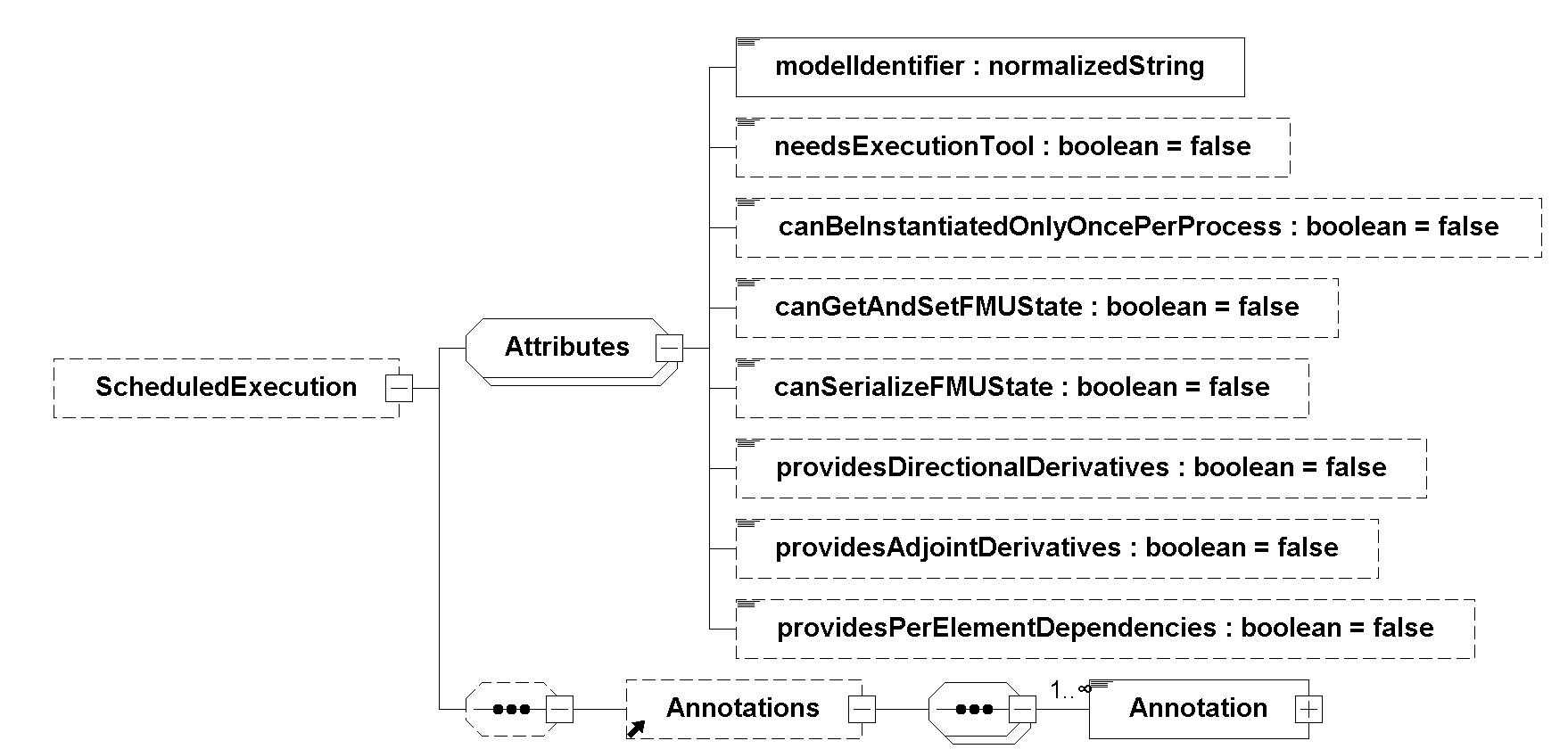
The element <ScheduledExecution> does not have any attributes other than defined as common attributes.
5.4.1. Example Model Description File
The simulation algorithm collects the information about the number and properties of Clocks supported by the FMU via analyzing the modelDescription.xml.
For every input Clock the simulation algorithm identifies a model partition of the FMU.
The properties intervalDecimal (or intervalCounter) and priority are defined based on the input clocks' intervalDecimal (or intervalCounter) and priority defined in the modelDescription.xml.
The simulation algorithm can read from the modelDescription.xml that output Clock OutClock may tick triggered by input Clock 10msClock and that input Clock AperiodicClock is triggered by OutClock.
<?xml version="1.0" encoding="UTF-8"?>
<fmiModelDescription fmiVersion="3.0" modelName="ThreeInputClocks" instantiationToken="ThreeInputClocks">
	<ScheduledExecution modelIdentifier="ThreeInputClocks"/>
	<LogCategories>
		<Category name="logStatusError" description="Log error messages"/>
	</LogCategories>
	<DefaultExperiment startTime="0" stopTime="6" stepSize="0.001"/>
	<ModelVariables>
		<!-- Variables related to input clock 10msClock  -->
		<Float64 name="AIn1" valueReference="0" causality="input" variability="discrete" clocks="5"
		start="0"/>
		<Float64 name="AIn2" valueReference="1" causality="input" variability="discrete" clocks="5"
		start="0"/>
		<Float64 name="AOut" valueReference="2" causality="output" variability="discrete" clocks="5"/>

		<!-- Variables related to input clock AperiodicClock  -->
		<Float64 name="BIn"  valueReference="3" causality="input" variability="discrete" clocks="6"
		start="0"/>
		<Float64 name="BOut" valueReference="4" causality="output" variability="discrete" clocks="6"/>

		<!-- Clock variables -->
		<!-- Periodic input clock -->
		<Clock name="10msClock" valueReference="5" causality="input" intervalVariability="constant"
		priority="1" intervalDecimal="0.01"/>
		<!-- Input clock that is triggered by 10msClock -->
		<Clock name="AperiodicClock" valueReference="6" causality="input" intervalVariability="countdown"
		priority="2" clocks="5"/>
		<!-- Output clock -->
		<Clock name="OutputClock" valueReference="7" causality="output" intervalVariability="triggered"
		clocks="5"/>
		<!-- Periodic input clock -->
		<Clock name="50msClock" valueReference="8" causality="input" intervalVariability="constant"
		priority="3" intervalDecimal="0.05"/>
	</ModelVariables>
	<ModelStructure>
		<Output valueReference="2" dependencies="0 1 5"/>
		<Output valueReference="4" dependencies="3 6"/>
		<Output valueReference="7" dependencies="5"/>
	</ModelStructure>
</fmiModelDescription>
References
-
[ABL12] Åkesson J., Braun W., Lindholm P., and Bachmann B. (2012): Generation of Sparse Jacobians for the Functional Mockup Interface 2.0. 9th International Modelica Conference, Munich, 2012. http://www.ep.liu.se/ecp/076/018/ecp12076018.pdf
-
[BPRS15] Atilim Gunes Baydin, Barak A. Pearlmutter, Alexey Andreyevich Radul, Jeffrey Mark Siskind (2015): Automatic differentiation in machine learning: a survey. https://www.jmlr.org/papers/volume18/17-468/17-468.pdf
-
[BCP10] Benveniste A., Caillaud B., Pouzet M. (2010): The Fundamentals of Hybrid Systems Modelers. In 49th IEEE International Conference on Decision and Control (CDC), Atlanta, Georgia, USA, December 15-17. http://www.di.ens.fr/~pouzet/bib/cdc10.pdf
-
[BOA11] Blochwitz T., Otter M., Arnold M., Bausch C., Clauß C., Elmqvist H., Junghanns A., Mauss J., Monteiro M., Neidhold T., Neumerkel D., Olsson H., Peetz J.-V., Wolf S. (2011): The Functional Mockup Interface for Tool independent Exchange of Simulation Models. 8th International Modelica Conference, Dresden 2011. http://www.ep.liu.se/ecp/063/013/ecp11063013.pdf
-
[BKF17] Braun W., Kulshreshtha K., Franke R., Walther A., Bachmann B., Towards Adjoint and Directional Derivatives in FMI utilizing ADOL-C within OpenModelica, 12th International Modelica Conference, Prague, 2017. https://2017.international.conference.modelica.org/proceedings/html/submissions/ecp17132363_BraunKulshreshthaFrankeBachmannWalther.pdf
-
[BOA12] Blochwitz T., Otter M., Åkesson J., Arnold M., Clauß C., Elmqvist H., Friedrich M., Junghanns A., Mauss J., Neumerkel D., Olsson H., Viel A. (2012): Functional Mockup Interface 2.0: The Standard for Tool independent Exchange of Simulation Models. 9th International Modelica Conference, Munich, 2012. http://www.ep.liu.se/ecp/076/017/ecp12076017.pdf
-
[KS00] Kübler R., Schiehlen W. (2000): Two methods of simulator coupling. Mathematical and Computer Modeling of Dynamical Systems 6 pp. 93-113.
-
[LZ07] Lee E.A., Zheng H. (2007): Leveraging Synchronous Language Principles for Heterogeneous Modeling and Design of Embedded Systems. EMSOFT'07, September 30-October 3, Salzburg, Austria. https://ptolemy.berkeley.edu/publications/papers/07/unifying/LeeZheng_SRUnifying.pdf
-
[MS93] Mattsson S. E. and Söderlind G.: Index Reduction in Differential Algebraic Equations Using Dummy Derivatives. SIAM Journal on Scientific Computing, Vol. 14, No. 3, pp. 677692, 1993.
-
[MLS12] Modelica (2012): Modelica, A Unified Object-Oriented Language for Systems Modeling. Language Specification, Version 3.3, May 9, 2012. https://www.modelica.org/documents/ModelicaSpec33.pdf
-
[PZ06] Pouzet M. (2006): Lucid Synchrone. Version 3.0, Tutorial and Reference Manual. http://www.di.ens.fr/~pouzet/lucid-synchrone/
-
[CGM84] Coleman, Garbow, Moré (1984): Software for estimating sparse Jacobian matrices, ACM Transactions on Mathematical Software. TOMS , vol. 10, no. 3, pp. 346-347
-
[PW13] Preston-Werner, T. (2013): Semantic Versioning 2.0.0. https://semver.org/spec/v2.0.0.html
-
[FBH18] Fritzson D., Braun R. and Hartford J. (2018): Composite modelling in 3-D mechanics utilizing Transmission Line Modelling (TLM) and Functional Mock-up Interface (FMI). Modeling, Identification and Control, vol. 39, no. 3, pp. 179-190.
Appendix A: Glossary
| Term | Description |
|---|---|
argument |
Refers to a function parameter. Not to be confused with parameter. |
capability flag |
Capability flags are used to indicate to the importer what optional functionality the FMU supports. |
clock |
A variable to report events or trigger events or model partitions. |
clock tick |
When the Clock ticks an event is present, otherwise the event is absent. A Clock tick causes a Clock activation at that time instant, except for input Clock ticks in Scheduled Execution, which cause an activation of the associated model partition instead. |
communication points |
Time grid for data exchange between importer and FMU(s) in a (co-)simulation environment. |
communication step size |
Distance between two subsequent communication points. |
continuous-time instant |
See time instant. |
co-simulation |
Coupling of several simulation programs in order to compute the global behavior of a system that consists of several subsystems. The subsystems are coupled in the sense that the behavior of each subsystem depends on the behavior of the remaining subsystems, so that the co-simulation must be computed in a step-by-step fashion. Each simulation program is responsible for computing the behavior of a subsystem, using the outputs produced by the other simulation programs. Synonyms: dynamic mutual-exchange, simulator coupling, and coupled simulation. |
direct feedthrough |
Direct feedthrough describes that values of output variables depend directly on values of input variables. |
domain change |
Used instead of zero-crossing. Indicates the change of an event indicator from the domain \(\mathbf{z}_j > 0\) to the domain \(\mathbf{z}_j \leq 0\) or from \(\mathbf{z}_j \leq 0\) to \(\mathbf{z}_j > 0\). See Section 3.1.1. |
Dynamic State Selection is a method to solve differential algebraic equations (DAEs). The FMU checks whether the dynamically selected states are still numerically appropriate. If not, a new mapping between states and variables is computed. For details see [MS93]. |
|
ECU |
Electronic Control Unit (Microprocessor that is used to control a technical system). |
Something that occurs instantaneously at a specific time or when a specific condition occurs.
At an event in Model Exchange, numerical integration is suspended and variables may change their values discontinuously.
In Co-Simulation, an event may interrupt a |
|
A variable that changes sign exactly at an event. See event indicator. |
|
An importer can iteratively call |
|
exporter |
A program that creates an FMU. |
external scheduler |
See scheduler. |
feedthrough |
See direct feedthrough. |
FMI |
Functional Mock-up Interface: |
FMI functions |
The function of the FMI C-API. |
FMI for Co-Simulation |
Functional Mock-up Interface for Co-Simulation: |
FMI for Model Exchange |
Functional Mock-up Interface for Model Exchange: |
FMI for Scheduled Execution |
Functional Mock-up Interface for Scheduled Execution: |
FMU |
Functional Mock-up Unit: |
FMU clock |
See Clock. |
The tool that imports or loads one or more FMUs. Also called simulation environment, environment, calling environment, (co-)simulation algorithm, target platform, target environment, integrator (in ME). |
|
independent variable |
All variables are a function of this |
An input event occurs when a discrete input variable changes, a continuous input variable has a discontinuity or a |
|
integration algorithm |
The numerical algorithm to solve differential equations. |
integrator |
A software component, which implements an integration algorithm. |
interface |
General: An abstraction of a software component that describes its behavior without dealing with the internal implementation. Software components communicate with each other via interfaces. |
interface type |
One of the three FMI variants "Model Exchange", "Co-simulation" or "Scheduled execution" |
machine epsilon |
Smallest floating point value. |
mock-up |
A full-sized structural, but not necessarily functional model built accurately to scale, used chiefly for study, testing, or display. In the context of computer aided design (CAD), a digital mock-up (DMU) means a computer-based representation of the product geometry with its parts, usually in 3-D, for all kinds of geometrical and mechanical analyses. |
model |
A model is a mathematical or logical representation of a system of entities, phenomena, or processes.
Basically a model is a simplified abstract view of the complex reality. |
model description file |
The model description file is an XML file named |
Model Description Schema |
An XML schema that defines how all relevant, non-executable, information about a "model class" (FMU) is stored in a text file in XML format.
Most important, data for every variable is defined (variable name, handle, data type, variability, unit, etc.), see |
An FMU may consist of several algorithms computing subsets of variables. A model partition is such an algorithm with variables connected to a Clock. The execution of a model partition is triggered by the activation of its Clock. |
|
ODE |
see Ordinary Differential Equation |
Ordinary Differential Equation |
Differential equation containing one or more functions of one independent variable (typically time) and the derivatives of those functions. |
output points |
Tool internal time grid for saving output data to file (in some tools also known as "communication points" - but this term is used in a different way in FMI for Co-Simulation, see above). |
output step size |
Distance between two subsequent output points. |
parameter |
A quantity within a model, which remains constant during simulation ( |
runtime environment |
See co-simulation environment |
simulation |
Compute the behavior of one or several models under specified conditions. |
simulation model |
see model |
simulation program |
Software to develop and/or solve simulation models.
The software includes a solver, may include a user interface and methods for post processing (see also: simulation tool, simulation environment). |
simulation tool |
see simulation program |
simulator |
A simulator can include one or more simulation programs. |
simulator coupling |
See tool coupling. |
solver |
Software component, which includes algorithms to solve models, for example, integration algorithms and event handling methods. |
state |
The continuous states of a model are all variables that appear differentiated in the model and are independent from each other. |
state event |
The time of state events is not known apriori. Event indicators are used to allow the importer finding the time of these state events precisely. |
Event that might occur at a completed integrator step signaled by calling |
|
structural parameter |
A parameter influencing the size and/or dimensionality of an array variable of an FMU. |
A precise definition of time taking into account iterations at an event.
For an FMU, the |
|
super-dense time instant |
See time instant and super-dense time. |
Event that is defined by a predefined time instant. Since the time instant is known in advance, the integrator can select its step size so that the event point is directly reached. Therefore, this event can be handled efficiently. |
|
A moment in time, either a continuous-time instant \(t = t_R\), or a super-dense time instant \(t = (t_R, t_I)\), see also super-dense time. |
|
A mathematical method which uses physically motivated time delays to decouple an equation system into independent parts during a specified time frame without compromising numerical stability. Also known as the bi-lateral delay line method. For more details see [FBH18]. |
|
user interface |
The part of the simulation program that gives the user control over the simulation and allows watching results. |
XML |
eXtensible Markup Language (www.w3.org/XML, en.wikipedia.org/wiki/XML) - An open standard to store information in text files in a structured form. |
Appendix B: Acknowledgements
Until Dec. 2011, this work was carried out within the ITEA2 MODELISAR project (project number: ITEA2-07006, https://itea3.org/project/modelisar.html).
Daimler AG, DLR, ITI GmbH, Martin Luther University Halle-Wittenberg, QTronic GmbH and SIMPACK AG thank BMBF for partial funding of this work within MODELISAR (BMBF Förderkennzeichen: 01lS0800x).
Dassault Systèmes (Sweden) thanks the Swedish funding agency VINNOVA (2008-02291) for partial funding of this work within MODELISAR.
LMS Imagine and IFPEN thank DGCIS for partial funding of this work within MODELISAR.
Since Sept. 2012 until Nov. 2015, this work is partially carried out within the ITEA2 MODRIO project (project number: ITEA 2-11004, https://itea3.org/project/modrio.html).
-
DLR, ITI GmbH, QTronic GmbH and SIMPACK AG thank BMBF for partial funding of this work within MODRIO (BMBF Förderkennzeichen: 01IS12022E).
-
Dassault Systèmes (Sweden), Linköping University and Modelon AB thank the Swedish funding agency VINNOVA (2012—01157) for partial funding of this work within MODRIO.
-
Siemens PLM Software (France) and IFPEN thank DGCIS for partial funding of this work within MODRIO.
-
Contributions of ESI Group were carried out within the project FMI4BIM, funded by the German Federal Ministry for Economic Affairs and Energy.
-
Dassault Systèmes (France) and EDF (France) thank BPIFrance and Region Ile de France for partially funding this work within ModeliScale project.
Appendix C: Contributors
The Modelica Association Project FMI was headed by Andreas Junghanns (Synopsys) and Torsten Blochwitz (ESI Group). The FMI 3.0 standard text is based on FMI 2.0 and FMI 1.0 and we wish to acknowledge their contributors.
Special thanks to
-
Andreas Junghanns (Synopsys) and Torsten Sommer (Dassault Systèmes) for the initial conversion of the FMI 2.0 Word document to AsciiDoc
-
Torsten Sommer (Dassault Systèmes) for the creation of the Reference FMUs and the Continuous Integration pipeline
-
Cláudio Gomes (Aarhus University) for the creation of the tooling to create the graphical representation of the XML schemas
-
Andreas Junghanns (Synopsys) and Torsten Blochwitz (ESI Group) for restructuring and re-writing the whole FMI standard text
-
all companies and organizations that participated in the FMI 3.0 Plugfests:
-
Aarhus University with VDMCheck
-
Altair with Activate
-
Augsburg University with FMI.jl
-
AVL List GmbH with Model.CONNECT™
-
Dassault Systèmes with Dymola, FMPy, and FMI Kit for Simulink
-
dSPACE GmbH with TargetLink, SystemDesk, ConfigurationDesk, and VEOS
-
ESI Group with SimulationX
-
ETAS GmbH with COSYM
-
Julia Computing with JuliaSim
-
Maplesoft with MapleSIM
-
OSMC
-
PMSF IT Consulting with FMI Bench
-
Synopsys with Silver
-
TLK-Thermo GmbH
-
The essential parts of the design of this version were developed by (alphabetical list)
-
Christian Bertsch, Robert Bosch GmbH, Germany
-
Matthias Blesken, dSPACE GmbH, Germany
-
Torsten Blochwitz, ESI Group, Germany
-
Cláudio Gomes, Aarhus University, Denmark
-
Andreas Junghanns, Synopsys, Germany
-
Pierre R. Mai, PMSF IT Consulting, Germany
-
Masoud Najafi, Altair, France
-
Andreas Pillekeit, dSPACE GmbH, Germany
-
Klaus Schuch, AVL List GmbH, Austria
-
Christian Schulze, TLK-Thermo GmbH, Germany
-
Torsten Sommer, Dassault Systèmes, Germany
-
Karl Wernersson, Dassault Systèmes, Sweden
-
Irina Zacharias, dSPACE GmbH, Germany
Additionally the following partners participated in FMI design meetings and contributed to the discussion (alphabetical list)
-
Nick Battle, United Kingdom
-
Martin Benedikt, Virtual Vehicle, Austria
-
Jorge Bernal-Romero, ITK-Engineering, Germany
-
Thomas Beutlich, previously at ESI Group, Germany
-
Robert Braun, Linköping University, Sweden
-
Paul Filip, Synopsys, Romania
-
Rüdiger Franke, ABB AG, Germany
-
Markus Friedrich, Dassault Systèmes, Germany
-
Thorsten Gehrmann, Fraunhofer IEM, Germany
-
Jan Niklas Jaeschke, TLK-Thermo, Germany
-
Oliver Kotte, Robert Bosch GmbH, Germany
-
Kaska Kowalalska, Maplesoft, Canada
-
Gunter Lantzsch, ESI Group, Germany
-
Timo Penndorf, ETAS GmbH, Germany
-
Tim Schenk, Siemens AG, Germany
-
Patrick Täuber, dSPACE GmbH, Germany
-
Jean-Philipp Tavella, EDF, France
-
Adrian Tirea, Synopsys, Romania
-
Otto Tronarp, Wolfram MathCore, Sweden
-
Antoine Viel, Siemens PLM, France